Last time, I used the implementation of MULTISPATI PCA in adespatial on the mouse skeletal muscle Visium dataset. The dataset is small by scRNA-seq standards, with only 900 something spots. It too about half a minute to run MULTISPATI PCA, to obtain 30 PCs with the most positive eigenvalues and 30 with the most negative eigenvalues. It might not sound too bad, but it only took less than one second to run non-spatial PCA with the IRLBA algorithm to obtain 30 PCs.

The adespatial implementation is slow because it performs full spectrum decomposition twice, with base R’s eigen() function. The first is to perform non-spatial PCA, whose output contains row and column weights and the original data that are then used by the multispati() function. The second time is for the spatially weighted covariance matrix in multispati(). Although only the top 30 positive and negative eigenvalues and their corresponding eigenvectors are retained in the results, all the 900 something eigenvalues and eigenvector were computed, doing a lot of unnecessary work.

I would like to perform MULTISPATI PCA on single cell resolution datasets with over 100,000 cells, so I need a more efficient implementation, which is what I do here.

Here we load the packages. Note that the devel version of SpatialFeatureExperiment and Voyager are used here.

library(Voyager)
library(ade4)
library(adespatial)
library(SFEData)
library(RSpectra)
library(tidyverse)
library(bench)
library(sf)
library(scater)
library(scran)
library(profvis)
library(spdep)
library(Matrix)
theme_set(theme_bw())

packageVersion("SpatialFeatureExperiment")

[1] '1.1.5'

packageVersion("Voyager")

[1] '1.1.10'

Dataset

The dataset used here is a MERFISH dataset from healthy mouse liver from Vizgen. It is available in the SFEData package.

(sfe <- VizgenLiverData())

snapshotDate(): 2022-10-31

see ?SFEData and browseVignettes('SFEData') for documentation

loading from cache

require("SpatialFeatureExperiment")

class: SpatialFeatureExperiment 
dim: 385 395215 
metadata(0):
assays(1): counts
rownames(385): Comt Ldha ... Blank-36 Blank-37
rowData names(3): means vars cv2
colnames(395215): 10482024599960584593741782560798328923
  111551578131181081835796893618918348842 ...
  92389687374928708938472537234969690424
  96399783859933548456002372694492036651
colData names(9): fov volume ... nCounts nGenes
reducedDimNames(0):
mainExpName: NULL
altExpNames(0):
spatialCoords names(2) : center_x center_y
imgData names(1): sample_id

Geometries:
colGeometries: centroids (POINT), cellSeg (POLYGON) 

Graphs:
sample01:

Plot cell density in histological space:

plotCellBin2D(sfe, bins = 300)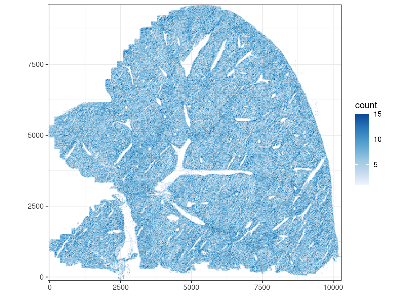

The cells are fairly uniformly distributed in space, but some structure with higher cell density, perhaps related to blood vessels, can be discerned.

QC was already performed in the Voyager MERFISH vignette so I won’t go into details here. I remove low quality cells that have too many transcript counts from the blank probes as I did in that vignette.

is_blank <- str_detect(rownames(sfe), "^Blank-")
sfe <- addPerCellQCMetrics(sfe, subset = list(blank = is_blank))

get_neg_ctrl_outliers <- function(col, sfe, nmads = 3, log = FALSE) {
    inds <- colData(sfe)$nCounts > 0 & colData(sfe)[[col]] > 0
    df <- colData(sfe)[inds,]
    outlier_inds <- isOutlier(df[[col]], type = "higher", nmads = nmads, log = log)
    outliers <- rownames(df)[outlier_inds]
    col2 <- str_remove(col, "^subsets_")
    col2 <- str_remove(col2, "_percent$")
    new_colname <- paste("is", col2, "outlier", sep = "_")
    colData(sfe)[[new_colname]] <- colnames(sfe) %in% outliers
    sfe
}

sfe <- get_neg_ctrl_outliers("subsets_blank_percent", sfe, log = TRUE)
(sfe <- sfe[, !sfe$is_blank_outlier & sfe$nCounts > 0])

class: SpatialFeatureExperiment 
dim: 385 390348 
metadata(0):
assays(1): counts
rownames(385): Comt Ldha ... Blank-36 Blank-37
rowData names(3): means vars cv2
colnames(390348): 10482024599960584593741782560798328923
  111551578131181081835796893618918348842 ...
  92389687374928708938472537234969690424
  96399783859933548456002372694492036651
colData names(16): fov volume ... total is_blank_outlier
reducedDimNames(0):
mainExpName: NULL
altExpNames(0):
spatialCoords names(2) : center_x center_y
imgData names(1): sample_id

Geometries:
colGeometries: centroids (POINT), cellSeg (POLYGON) 

Graphs:
sample01:

# Remove the blanks
sfe <- sfe[!is_blank,]

Normalize the data:

sfe <- logNormCounts(sfe)

Because this dataset only has 385 curated genes, it’s unnecessary to find highly variable genes.

Implementation

To recap, MULTISPATI diagonalizes a symmetric matrix

\[ H = \frac 1 {2n} X(W^t+W)X^t, \]

where \(X\) denotes a gene count matrix whose columns are cells or Visium spots and whose rows are genes, with \(n\) columns. \(W\) is the row normalized \(n\times n\) adjacency matrix of the spatial neighborhood graph of the cells or Visium spots, which does not have to be symmetric.

There’re over 390,000 cells and I’ll use a small subset to test the implementation before a more systematic benchmark.

bbox <- st_as_sfc(st_bbox(c(xmin = 6500, ymin = 3750, xmax = 7000, ymax = 4250)))
inds <- st_intersects(centroids(sfe), bbox, sparse = FALSE)
(sfe_sub <- sfe[,inds])

class: SpatialFeatureExperiment 
dim: 347 1425 
metadata(0):
assays(2): counts logcounts
rownames(347): Comt Ldha ... Pdha2 Hsd17b3
rowData names(3): means vars cv2
colnames(1425): 1090737716093966147093269971771778743
  116394482990407538610204487800212441420 ...
  300214274088721611056184746460936395547
  336480762885429101958042577061602745945
colData names(17): fov volume ... is_blank_outlier sizeFactor
reducedDimNames(0):
mainExpName: NULL
altExpNames(0):
spatialCoords names(2) : center_x center_y
imgData names(1): sample_id

Geometries:
colGeometries: centroids (POINT), cellSeg (POLYGON) 

Graphs:
sample01:

Plot the cells of this subset:

plotGeometry(sfe_sub, "cellSeg")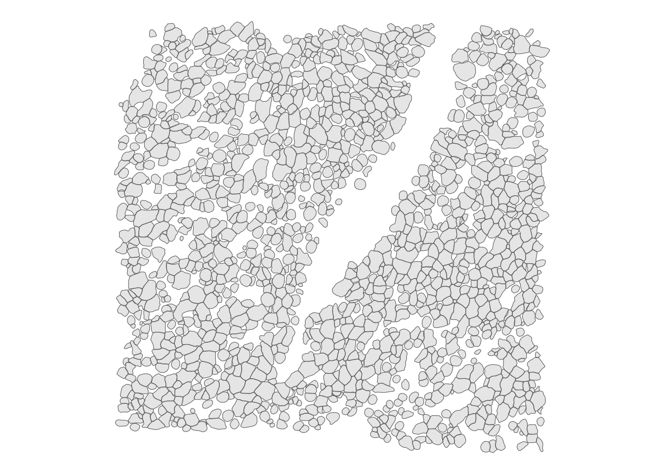

Most tessellations of the 2D plane in real data are somewhere between a square (4 rook neighbors) and a hexagonal (6 neighbors) grid. Uncertainties in cell segmentation means that cell segmentation polygon contiguity might have many false negatives so a polygon contiguity graph may miss many actual neighbors. Hence we use the k nearest neighbor method to find a spatial neighborhood graph, with \(k = 5\), which appears reasonable from visual inspections. Furthermore, k nearest neighbor is more scalable to larger datasets compared to some other methods such as triangulation following by edge pruning. The devel (Bioconductor 3.17) version of SpatialFeatureExperiment can find k nearest neighbors much more efficiently than the release (Bioconductor 3.16) version. Inverse distance weighting is used so neighbors further away have less contribution, and the weighted spatial neighborhood adjacency matrix is row normalized as is customary for MULTISPATI and default in spdep so the spatially lagged values are comparable to the original values.

colGraph(sfe_sub, "knn") <- findSpatialNeighbors(sfe_sub, method = "knearneigh", 
                                                 k = 5, dist_type = "idw", 
                                                 style = "W")

Here we plot the spatial neighborhood graph, where transparency of the edges corresponds to edge weight:

plotColGraph(sfe_sub, "knn", colGeometryName = "centroids", weights = TRUE) +
    theme_void()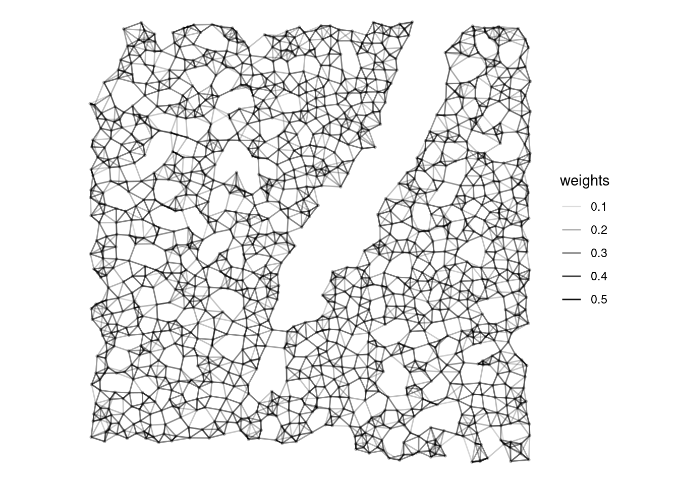

Wrapping everything needed to get MULTISPATI results from adespatial ready to be added to reducedDims(sfe_sub) in one function:

calc_multispati_ade <- function(sfe, colGraphName, nfposi = 30, nfnega = 30) {
    df <- logcounts(sfe) |> # Don't need highly variable genes here
        as.matrix() |> t() |> 
        as.data.frame()
    pca <- dudi.pca(df, scannf = FALSE, nf = nfposi) # scales data by default
    multispati_res <- multispati(pca, colGraph(sfe, colGraphName), scannf = FALSE,
                             nfposi = nfposi, nfnega = nfnega)
    multispati_mat <- as.matrix(multispati_res$li)
    rownames(multispati_mat) <- colnames(sfe)
    loadings <- as.matrix(multispati_res$c1)
    rownames(loadings) <- rownames(sfe)
    colnames(loadings) <- str_replace(colnames(loadings), "CS", "PC")
    attr(multispati_mat, "rotation") <- loadings
    attr(multispati_mat, "eig") <- multispati_res$eig
    multispati_mat
}

Here I use profvis to profile the code, to see the time and memory taken by each function called:

profvis({ade_res <- calc_multispati_ade(sfe_sub, "knn")})

This usually takes from 50 seconds to about a minute and 200 to 300 something MB of RAM on my lab’s server where R does NOT use an optimized BLAS (the results would be slightly different every time I run it). According to the profile, the vast majority of time was spent on eigen(), which was called twice and performed the full eigen decomposition, although only a small subset of eigenvectors are retained in the results.

I ran the same code on my laptop which uses the optimized Apple vecLib BLAS. My laptop is a 2017 MacBook Pro with 8 GB of RAM and 2 physical CPU cores. The adespatial implementation took 390 ms (eigen() used 30 ms) and 257.5 MB of RAM. Using an optimized BLAS drastically speeds up matrix operations. See this page for instructions on changing to an optimized BLAS in Ubuntu. For Fedora, it’s possible to change BLAS without leaving the R session with flexiblas. For Mac, R 4.2 comes with vecLib so you no longer have to locate the vecLib from the system. Here’s the official instruction for Mac to make R use vecLib. Unfortunately, from my online search as I don’t personally use Windows, there is no better option than Microsoft R Open for Windows.

Here is my implementation of MULTISPATI, with everything I can do to improve efficiency I can think of. In the spdep package, the listw2mat() function converts a listw spatial neighborhood graph object into an adjacency matrix, but it’s a dense matrix with mostly 0’s, so using a sparse matrix will save memory.

# Convert listw to sparse matrix to save memory
listw2sparse <- function(listw) {
    i <- rep(seq_along(listw$neighbours), times = card(listw$neighbours))
    j <- unlist(listw$neighbours)
    x <- unlist(listw$weights)
    sparseMatrix(i = i, j = j, x = x)
}

Then wrap everything needed to get MULTISPATI results ready to be added to reducedDims(sfe_sub) in one function:

# nf positive and negative eigenvalues
calc_multispati_rspectra <- function(sfe, colGraphName, nf = 30) {
    # Scaled matrix is no longer sparse
    X <- as.matrix(t(logcounts(sfe)))
    X <- sweep(X, 2, colMeans(X))
    # Note that dudi.pca divides by n instead of n-1 when scaling data
    n <- nrow(X)
    X <- sweep(X, 2, sqrt(colVars(X)*(n-1)/n), FUN = "/")
    W <- listw2sparse(colGraph(sfe, colGraphName))
    mid <- W + t(W)
    covar <- t(X) %*% mid %*% X / (2*nrow(X))
    res <- eigs_sym(covar, k = nf * 2, which = "BE")
    loadings <- res$vectors
    out <- X %*% loadings
    colnames(out) <- paste0("PC", seq_len(ncol(out)))
    attr(out, "rotation") <- loadings
    attr(out, "eig") <- res$values
    out
}

I noted that ade4::dudi.pca(), whose output is used in multispati(), divides by n when computing the variance when scaling the data. This is the maximum likelihood estimate, while dividing by n-1 is the unbiased estimate. Shall I use n or n-1? For the typical size of spatial transcriptomics data, this shouldn’t cause very much of a difference

Again, I profile this run:

profvis({rsp_res <- calc_multispati_rspectra(sfe_sub, "knn")})

This usually takes 500 something ms and around 40 MB of RAM, without optimized BLAS. It is indeed much faster than the adespatial implementation, over 80 times faster. Much of the time was spent on matrix multiplication. On my laptop with vecLib, this took 90 ms and 42.5 MB of RAM, over 4 times faster than the adespatial implementation run with vecLib. Using vecLib does not reduce memory usage.

Now check if the results are the same:

# Eigenvalues
all.equal(head(attr(rsp_res, "eig"), 30), head(attr(ade_res, "eig"), 30))

[1] TRUE

all.equal(tail(attr(rsp_res, "eig"), 30), tail(attr(ade_res, "eig"), 30))

[1] TRUE

So the eigenvalues are the same. Plot the eigenvalues:

plot(attr(rsp_res, "eig"), ylab = "Eigenvalue")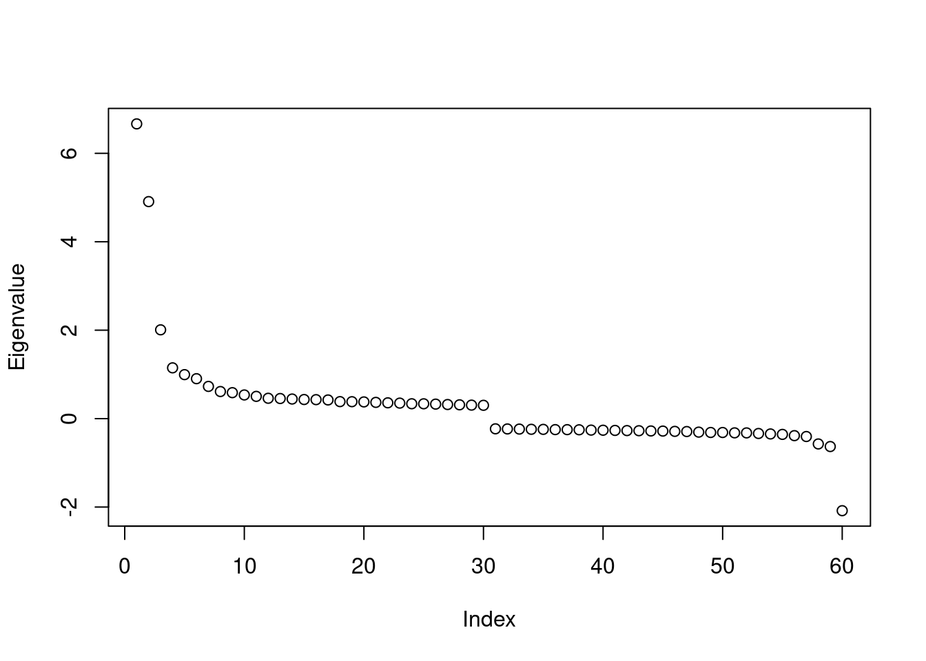

Note that unlike in non-spatial PCA, the eigenvalues here don’t correspond to variance explained. Rather, it’s the product of variance explained and Moran’s I of the eigenvector. The eigenvalue drops sharply from PC1 to PC4, then levels off after PC7. The most negative eigenvalue is about -2 and the absolute value drops sharply in the next most negative eigenvalue. Given the magnitude of the eigenvalue, the most negative eigenvector might be interesting, as the Voyager MERFISH vignette hints at the presence of negative spatial autocorrelation in this dataset at the cellular level, as Moran’s I for total transcript counts per cell is somewhat negative, at around -0.1, which might not be weak given that the lower bound of Moran’s I given the spatial neighborhood graph is usually closer to -0.5 than -1, while the upper bound is usually approximately 1.

Also note that spatial autocorrelation in datasets with single cell resolution should be interpreted differently from that in Visium which does not have single cell resolution, because of different length scales. In a geographical analogy, this is just like comparing houses as opposed to comparing neighborhoods, or comparing cities as opposed to comparing states.

Then we compare the eigenvectors, allowing for flipping (i.e. multiplied by -1), which is OK, because an eigenvector multiplied by a scalar is still an eigenvector of the same matrix with the same eigenvalue.

plot_pc_diffs <- function(mat1, mat2, npcs = 30, tail = FALSE, title = NULL) {
    diffs <- numeric(npcs)
    if (tail) {
        ind1 <- tail(seq_len(ncol(mat1)), npcs)
        ind2 <- tail(seq_len(ncol(mat2)), npcs)
    } else {
        ind1 <- ind2 <- seq_len(npcs)
    }
    for (i in seq_len(npcs)) {
        pc1 <- mat1[,ind1[i]]
        pc2 <- mat2[,ind2[i]]
        diffs[i] <- min(mean(abs(pc1 - pc2)), mean(abs(pc1 + pc2))) # flipped
    }
    tibble(difference = diffs,
           PC = seq_len(npcs)) |> 
        ggplot(aes(PC, difference)) +
        geom_line() +
        geom_hline(yintercept = sqrt(.Machine$double.eps), linetype = 2) +
        scale_y_log10() +
        scale_x_continuous(breaks = scales::breaks_width(5)) +
        annotation_logticks(sides = "l") +
        labs(title = title, y = "Mean absolute difference")
}

Compare the eigenvectors with positive eigenvalues:

plot_pc_diffs(attr(rsp_res, "rotation"), attr(ade_res, "rotation"),
              title = "Differences in eigenvectors, adespatial vs. RSpectra, positive")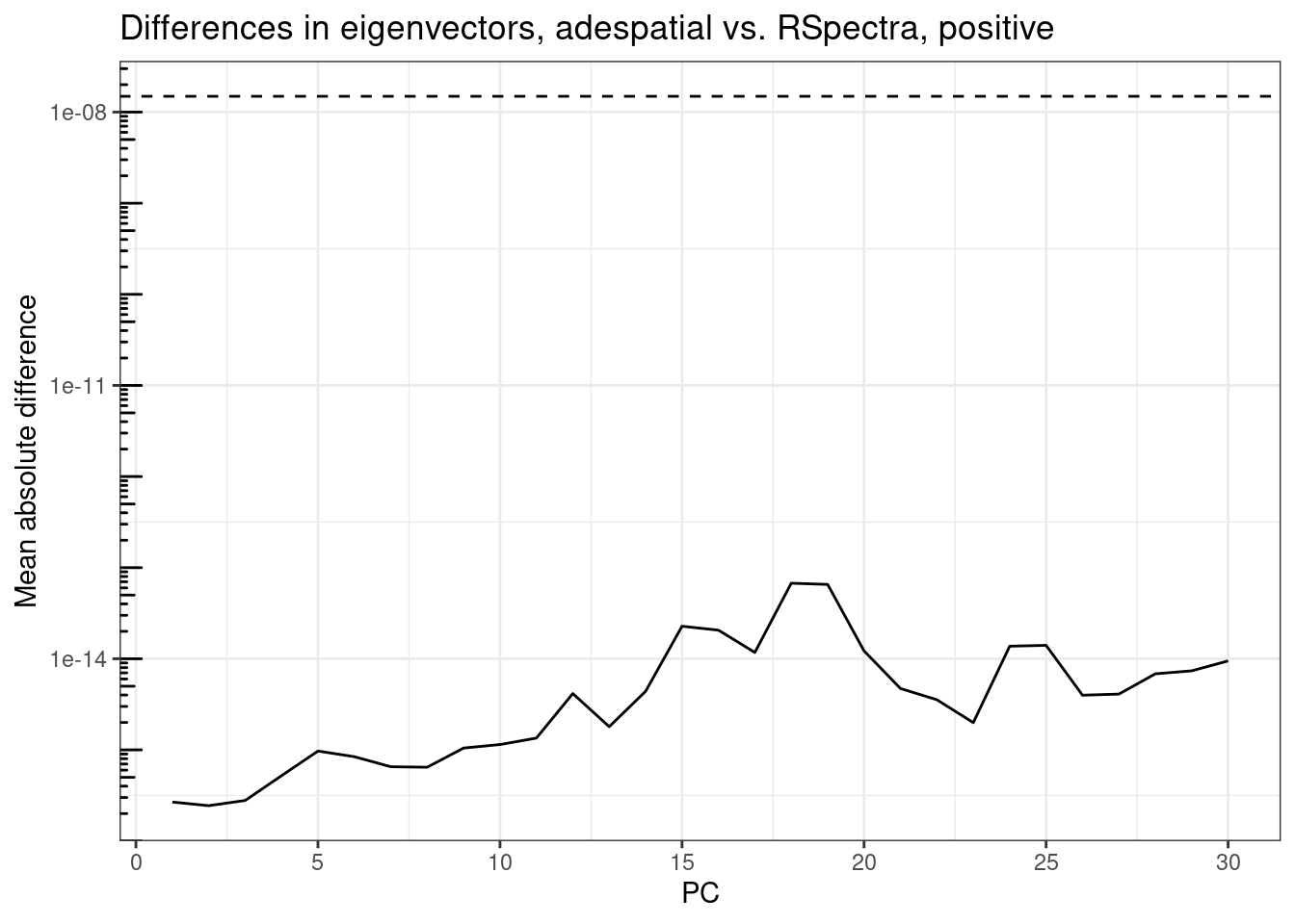

Compare the eigenvectors with negative eigenvalues:

plot_pc_diffs(attr(rsp_res, "rotation"), attr(ade_res, "rotation"), tail = TRUE,
              title = "Differences in eigenvectors, adespatial vs. RSpectra, negative")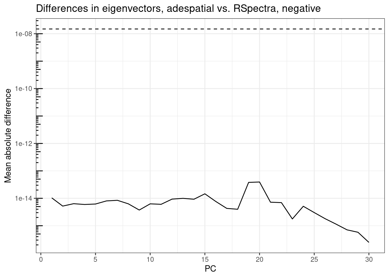

The differences are well below epsilon for all 30 PCs on both ends of the spectrum, mostly below 1e-14, i.e. can be accounted for by machine precision (the dashed line around 1.5e-8). The difference somewhat increases for eigenvalues with smaller absolute values, but still well below epsilon.

Compare the cell embeddings, first for positive eigenvalues: In theory, because the eigenvectors are the same (allowing for flipping) and the embeddings are found by the dot product of the gene expression profile of each cell with each PC, the embeddings should be the same. However, I’m plotting the differences here just in case adespatial does something extra behind the scene.

plot_pc_diffs(rsp_res, ade_res,
              title = "Differences in embeddings, adespatial vs. RSpectra, positive")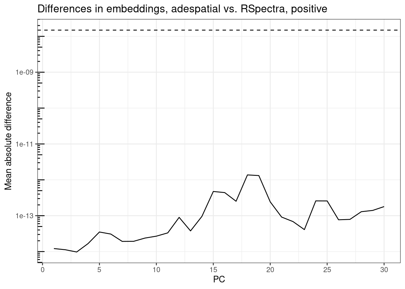

plot_pc_diffs(rsp_res, ade_res, tail = TRUE,
              title = "Differences in embeddings, adespatial vs. RSpectra, negative")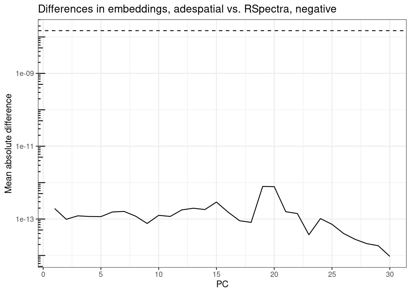

The embeddings are also well below epsilon and the differences have the same patterns as those of eigenvectors, so adespatial simply computed the dot product without doing anything else. So in conclusion, my RSpectra implementation gives consistent results as the adespatial implementation but 80 times faster without optimized BLAS and 4 times faster with optimized BLAS.

That said, the adespatial implementation allows for different column and row weighting for other types of duality diagram multivariate analyses. For now, I’m only concerned with PCA, so my implementation is simplified.

Benchmark

Since the default is non-optimized BLAS and those using a server most likely can’t change the BLAS, I perform the benchmark without optimized BLAS. I use different sized bounding boxes to spatially subset the data and compare the time and memory usage of the two implementations of MULTISPATI, with 30 most positive and 30 most negative eigenvalues. This dataset has 385 genes, which should not make this benchmark irrelevant because in spatial transcriptomics, the datasets with the most cells come from smFISH based methods such as MERFISH, which typically have a few hundred curated genes. Transcriptome wide datasets with hundreds of thousands of cells or spots are less common, but with subcellular NGS based methods such as PIXEL-seq and Stereo-seq, these datasets may be coming. MULTISPATI is a spatial method.

Here I get the sizes of boxes spanning orders of magnitude, to get a wide range of numbers of cells:

(diffs <- 2^seq(7, 13, length.out = 7))

[1]  128  256  512 1024 2048 4096 8192

Here I run the benchmark using the different sized subsets. I’m not checking if the results match here as is default in bench::mark(), because I have already checked, and because the eigenvectors can be flipped so the comparison is more involved than all.equal(). Both time and memory usage are recorded.

benchmark_multispati <- function(sfe, diff) {
    xmin <- 3000
    ymin <- 3000
    bbox <- st_as_sfc(st_bbox(c(xmin = xmin, ymin = ymin, 
                                xmax = xmin + diff, ymax = ymin + diff)))
    inds <- st_intersects(centroids(sfe), bbox, sparse = FALSE)
    sfe_sub <- sfe[,inds]
    colGraph(sfe_sub, "knn") <- findSpatialNeighbors(sfe_sub, method = "knearneigh",
                                                     k = 5, dist_type = "idw", 
                                                     style = "W")
    df <- bench::mark(adespatial = calc_multispati_ade(sfe_sub, "knn"),
                      rspectra = calc_multispati_rspectra(sfe_sub, "knn"),
                      max_iterations = 1, check = FALSE)
    df$ncells <- ncol(sfe_sub)
    df
}

Reformat the results for plotting:

if (!file.exists("benchmark_res.rds")) {
    benchmark_res <- map_dfr(diffs, benchmark_multispati, sfe = sfe)
    benchmark_res <- benchmark_res |> 
        mutate(expression = as.character(expression),
               mem_alloc = as.numeric(mem_alloc)/(1024^2))
    saveRDS(benchmark_res, "benchmark_res.rds")
} else {
    benchmark_res <- readRDS("benchmark_res.rds")
}

# Get colorblind friendly palette
data("ditto_colors")

Here I plot the time taken vs. the number of cells for both implementations:

ggplot(benchmark_res, aes(ncells, total_time, color = expression)) +
    geom_line() +
    scale_x_log10() +
    annotation_logticks() +
    labs(x = "Number of cells", y = "Time", color = "Implementation") +
    scale_color_manual(values = ditto_colors)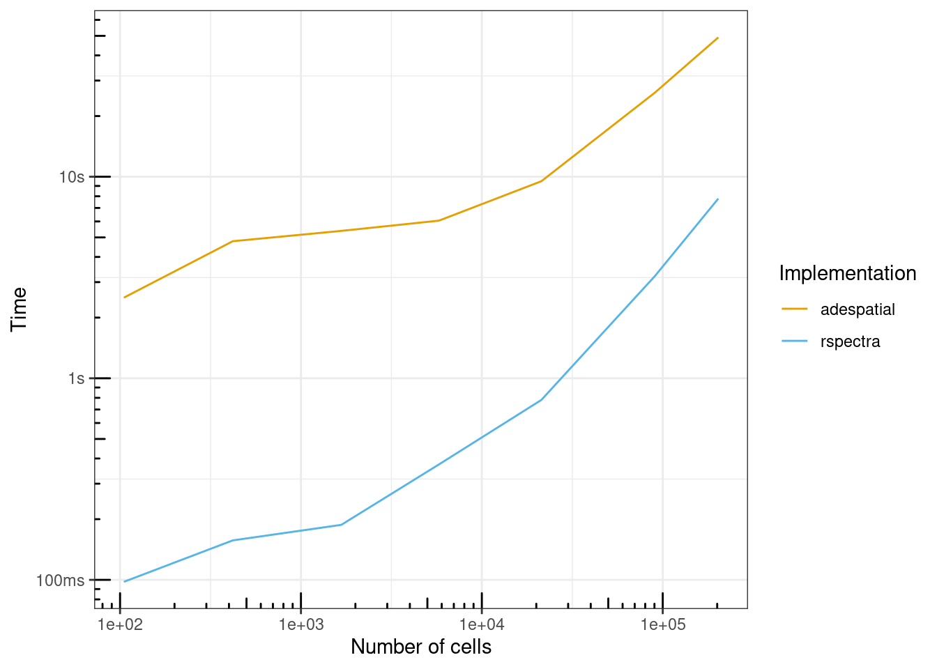

When run non-interactively in this benchmark, both implementations were much faster than the initial profiles above. But RSpectra is overall an order of magnitude faster than adespatial, though the gap shrinks with increasing number of cells, from over 20 times faster at around 100 cells to about 7 times faster at over 200,000 cells. For 200,000 cells, adespatial took 50 seconds when run non-interactively, while RSpectra took 7.79 seconds.

Also plot memory usage vs. number of cells:

ggplot(benchmark_res, aes(ncells, mem_alloc, color = expression)) +
    geom_line() +
    scale_x_log10() +
    scale_y_log10(breaks = scales::breaks_log()) +
    annotation_logticks() +
    labs(x = "Number of cells", y = "Memory (MB)", color = "Implementation") +
    scale_color_manual(values = ditto_colors)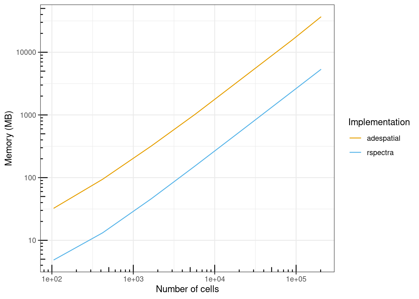

RSpectra also uses about 7 times less memory than adespatial across different number of cells. For the largest subset, with over 200,000 cells, adespatial used 36 GB of RAM, while RSpectra used about 5.2 GB, so while the latter can be run on my laptop, the former cannot.

So the RSpectra implementation of MULTISPATI looks promising. It will be added to Voyager for the Bioconductor 3.17 release. In addition, I should modify the PCA-related plotting functions in Voyager to improve user experiences around negative eigenvalues. In the sequel of this post, I’ll apply the now more scalable MULTISPATI PCA to the entire dataset with nearly 400,000 cells and try to do some biological interpretations.

Session info

sessionInfo()

R version 4.2.1 (2022-06-23)
Platform: x86_64-redhat-linux-gnu (64-bit)
Running under: CentOS Stream 8

Matrix products: default
BLAS/LAPACK: /usr/lib64/libopenblaso-r0.3.12.so

locale:
 [1] LC_CTYPE=en_US.UTF-8       LC_NUMERIC=C              
 [3] LC_TIME=en_US.UTF-8        LC_COLLATE=en_US.UTF-8    
 [5] LC_MONETARY=en_US.UTF-8    LC_MESSAGES=en_US.UTF-8   
 [7] LC_PAPER=en_US.UTF-8       LC_NAME=C                 
 [9] LC_ADDRESS=C               LC_TELEPHONE=C            
[11] LC_MEASUREMENT=en_US.UTF-8 LC_IDENTIFICATION=C       

attached base packages:
[1] stats4    stats     graphics  grDevices utils     datasets  methods  
[8] base     

other attached packages:
 [1] SpatialFeatureExperiment_1.1.5 Matrix_1.5-3                  
 [3] spdep_1.2-8                    spData_2.2.2                  
 [5] profvis_0.3.7                  scran_1.26.1                  
 [7] scater_1.27.3                  scuttle_1.8.4                 
 [9] SingleCellExperiment_1.20.1    SummarizedExperiment_1.28.0   
[11] Biobase_2.58.0                 GenomicRanges_1.50.2          
[13] GenomeInfoDb_1.34.9            IRanges_2.32.0                
[15] S4Vectors_0.36.2               BiocGenerics_0.44.0           
[17] MatrixGenerics_1.10.0          matrixStats_0.63.0            
[19] sf_1.0-12                      bench_1.1.2                   
[21] lubridate_1.9.2                forcats_1.0.0                 
[23] stringr_1.5.0                  dplyr_1.1.1                   
[25] purrr_1.0.1                    readr_2.1.4                   
[27] tidyr_1.3.0                    tibble_3.2.1                  
[29] ggplot2_3.4.1                  tidyverse_2.0.0               
[31] RSpectra_0.16-1                SFEData_1.1.1                 
[33] adespatial_0.3-21              ade4_1.7-22                   
[35] Voyager_1.1.10                

loaded via a namespace (and not attached):
  [1] utf8_1.2.3                    R.utils_2.12.2               
  [3] tidyselect_1.2.0              RSQLite_2.3.0                
  [5] AnnotationDbi_1.60.0          htmlwidgets_1.6.1            
  [7] grid_4.2.1                    BiocParallel_1.32.6          
  [9] RNeXML_2.4.11                 DropletUtils_1.18.1          
 [11] ScaledMatrix_1.6.0            munsell_0.5.0                
 [13] codetools_0.2-19              units_0.8-1                  
 [15] statmod_1.5.0                 interp_1.1-3                 
 [17] withr_2.5.0                   colorspace_2.1-0             
 [19] filelock_1.0.2                knitr_1.42                   
 [21] uuid_1.1-0                    rstudioapi_0.14              
 [23] wk_0.7.2                      labeling_0.4.2               
 [25] GenomeInfoDbData_1.2.9        farver_2.1.1                 
 [27] bit64_4.0.5                   rhdf5_2.42.0                 
 [29] vctrs_0.6.1                   generics_0.1.3               
 [31] xfun_0.37                     timechange_0.2.0             
 [33] BiocFileCache_2.6.1           adegenet_2.1.10              
 [35] adephylo_1.1-13               R6_2.5.1                     
 [37] ggbeeswarm_0.7.1              rsvd_1.0.5                   
 [39] locfit_1.5-9.7                bitops_1.0-7                 
 [41] rhdf5filters_1.10.0           cachem_1.0.7                 
 [43] DelayedArray_0.24.0           promises_1.2.0.1             
 [45] scales_1.2.1                  beeswarm_0.4.0               
 [47] gtable_0.3.3                  phylobase_0.8.10             
 [49] beachmat_2.14.0               rlang_1.1.0                  
 [51] splines_4.2.1                 scico_1.3.1                  
 [53] BiocManager_1.30.20           s2_1.1.2                     
 [55] yaml_2.3.7                    reshape2_1.4.4               
 [57] httpuv_1.6.9                  tools_4.2.1                  
 [59] SpatialExperiment_1.8.1       ellipsis_0.3.2               
 [61] RColorBrewer_1.1-3            proxy_0.4-27                 
 [63] Rcpp_1.0.10                   plyr_1.8.8                   
 [65] sparseMatrixStats_1.10.0      progress_1.2.2               
 [67] zlibbioc_1.44.0               classInt_0.4-9               
 [69] RCurl_1.98-1.10               prettyunits_1.1.1            
 [71] deldir_1.0-6                  viridis_0.6.2                
 [73] ggrepel_0.9.3                 cluster_2.1.4                
 [75] magrittr_2.0.3                magick_2.7.4                 
 [77] ggnewscale_0.4.8              hms_1.1.2                    
 [79] patchwork_1.1.2               mime_0.12                    
 [81] evaluate_0.20                 xtable_1.8-4                 
 [83] XML_3.99-0.13                 jpeg_0.1-10                  
 [85] gridExtra_2.3                 compiler_4.2.1               
 [87] KernSmooth_2.23-20            crayon_1.5.2                 
 [89] R.oo_1.25.0                   htmltools_0.5.4              
 [91] mgcv_1.8-42                   later_1.3.0                  
 [93] tzdb_0.3.0                    DBI_1.1.3                    
 [95] ExperimentHub_2.6.0           dbplyr_2.3.2                 
 [97] MASS_7.3-58.2                 rappdirs_0.3.3               
 [99] boot_1.3-28.1                 permute_0.9-7                
[101] cli_3.6.1                     adegraphics_1.0-18           
[103] R.methodsS3_1.8.2             metapod_1.6.0                
[105] parallel_4.2.1                igraph_1.4.1                 
[107] pkgconfig_2.0.3               rncl_0.8.7                   
[109] sp_1.6-0                      xml2_1.3.3                   
[111] vipor_0.4.5                   dqrng_0.3.0                  
[113] XVector_0.38.0                digest_0.6.31                
[115] vegan_2.6-4                   Biostrings_2.66.0            
[117] rmarkdown_2.20                edgeR_3.40.2                 
[119] DelayedMatrixStats_1.20.0     curl_5.0.0                   
[121] shiny_1.7.4                   rjson_0.2.21                 
[123] lifecycle_1.0.3               nlme_3.1-162                 
[125] jsonlite_1.8.4                Rhdf5lib_1.20.0              
[127] BiocNeighbors_1.16.0          seqinr_4.2-23                
[129] viridisLite_0.4.1             limma_3.54.2                 
[131] fansi_1.0.4                   pillar_1.9.0                 
[133] lattice_0.20-45               KEGGREST_1.38.0              
[135] fastmap_1.1.1                 httr_1.4.5                   
[137] interactiveDisplayBase_1.36.0 glue_1.6.2                   
[139] png_0.1-8                     bluster_1.8.0                
[141] BiocVersion_3.16.0            bit_4.0.5                    
[143] class_7.3-21                  stringi_1.7.12               
[145] HDF5Array_1.26.0              blob_1.2.4                   
[147] BiocSingular_1.14.0           AnnotationHub_3.6.0          
[149] latticeExtra_0.6-30           memoise_2.0.1                
[151] irlba_2.3.5.1                 e1071_1.7-13                 
[153] ape_5.7-1