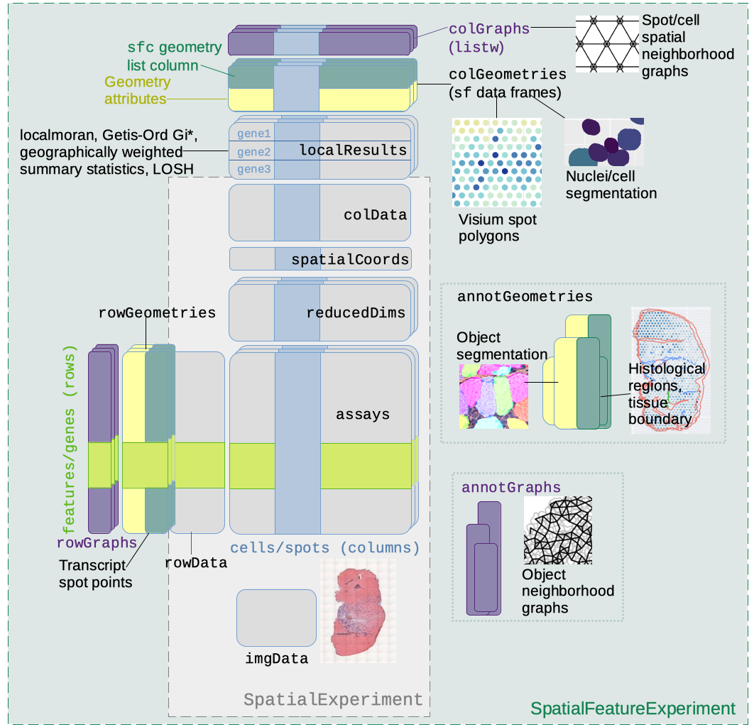
SpatialFeatureExperiment
SpatialFeatureExperiment (SFE) is a new S4 class built on top of SpatialExperiment
(SPE). SFE incorporates geometries and geometric operations with the sf
package. Examples of supported geometries are Visium spots represented
with polygons corresponding to their size, cell or nuclei segmentation
polygons, tissue boundary polygons, pathologist annotation of
histological regions, and transcript spots of genes. Using
sf, SpatialFeatureExperiment leverages the
GEOS C++ library underlying sf for geometry operations,
including algorithms for for determining whether geometries intersect,
finding intersection geometries, buffering geometries with margins, etc.
A schematic of the SFE object is shown below:
Below is a list of SFE features that extend the SPE object:
-
colGeometriesaresfdata frames associated with the entities that correspond to columns of the gene count matrix, such as Visium spots or cells. The geometries in thesfdata frames can be Visium spot centroids, Visium spot polygons, or for datasets with single cell resolution, cell or nuclei segmentations. MultiplecolGeometriescan be stored in the same SFE object, such as one for cell segmentation and another for nuclei segmentation. There can be non-spatial, attribute columns in acolGeometryrather thancolData, because thesfclass allows users to specify how attributes relate to geometries, such as “constant”, “aggregate”, and “identity”. See theagrargument of thest_sfdocumentation. -
colGraphsare spatial neighborhood graphs of cells or spots. The graphs have classlistw(spdeppackage), and thecolPairsofSingleCellExperimentwas not used so no conversion is necessary to use the numerous spatial dependency functions fromspdep, such as those for Moran’s I, Geary’s C, Getis-Ord Gi*, LOSH, etc. Conversion is also not needed for other classical spatial statistics packages such asspatialregandadespatial. -
rowGeometriesare similar tocolGeometries, but support entities that correspond to rows of the gene count matrix, such as genes. As we shall see below, a use case is to store transcript spots for each gene in smFISH or in situ sequencing based datasets. -
rowGraphsare similar tocolGraphs. A potential use case may be spatial colocalization of transcripts of different genes. -
annotGeometriesaresfdata frames associated with the dataset but not directly with the gene count matrix, such as tissue boundaries, histological regions, cell or nuclei segmentation in Visium datasets, and etc. These geometries are stored in this object to facilitate plotting and usingsffor operations such as to find the number of nuclei in each Visium spot and which histological regions each Visium spot intersects. UnlikecolGeometriesandrowGeometries, the number of rows in thesfdata frames inannotGeometriesis not constrained by the dimension of the gene count matrix and can be arbitrary. -
annotGraphsare similar tocolGraphsandrowGraphs, but are for entities not directly associated with the gene count matrix, such as spatial neighborhood graphs for nuclei in Visium datasets, or other objects like myofibers. These graphs are relevant tospdepanalyses of attributes of these geometries such as spatial autocorrelation in morphological metrics of myofibers and nuclei. With geometry operations withsf, these attributes and results of analyses of these attributes (e.g. spatial regions defined by the attributes) may be related back to gene expression. -
localResultsare similar toreducedDimsinSingleCellExperiment, but stores results from univariate and bivariate local spatial analysis results, such as fromlocalmoran, Getis-Ord Gi*, and local spatial heteroscedasticity (LOSH). Unlike inreducedDims, for each type of results (type is the type of analysis such as Getis-Ord Gi*), each feature (e.g. gene) or pair of features for which the analysis is performed has its own results. The local spatial analyses can also be performed for attributes ofcolGeometriesandannotGeometriesin addition to gene expression andcolData. Results of multivariate spatial analysis such as MULTISPATI PCA can be stored inreducedDims. -
imgDatastore images associated with the dataset. This field is inherited from SPE, but SFE has extended the image functionalities so images are not loaded into memory unless necessary.
Create an SFE object
Visium
10x Genomics Space Ranger output from a Visium experiment can be read
in a similar manner as in SpatialExperiment; the
SpatialFeatureExperiment SFE object has the
spotPoly column geometry for the spot polygons. If the
filtered matrix (i.e. only spots in the tissue) is read in, then a
column graph called visium will also be present for the
spatial neighborhood graph of the Visium spots on the tissue. The graph
is not computed if all spots are read in regardless of whether they are
on tissue.
dir <- system.file("extdata", package = "SpatialFeatureExperiment")
sample_ids <- c("sample01", "sample02")
(samples <- file.path(dir, sample_ids))
#> [1] "/usr/local/lib/R/site-library/SpatialFeatureExperiment/extdata/sample01"
#> [2] "/usr/local/lib/R/site-library/SpatialFeatureExperiment/extdata/sample02"
The results for each tissue capture should be in the
outs directory under the sample directory. Inside the
outs directory, these directories may be present:
raw_reature_bc_matrix has the unfiltered gene count matrix,
filtered_feature_bc_matrix has the gene count matrix for
spots in tissue, and spatial has the spatial information.
The matrix directories contain the matrices in MTX format as sparse
matrices. Space Ranger also outputs the matrices as h5 files, which are
read into R in a similar way as MTX.
list.files(file.path(samples[1], "outs"))
#> [1] "filtered_feature_bc_matrix" "spatial"
Inside the matrix directory:
list.files(file.path(samples[1], "outs", "filtered_feature_bc_matrix"))
#> [1] "barcodes.tsv" "features.tsv" "matrix.mtx"
Inside the spatial directory:
list.files(file.path(samples[1], "outs", "spatial"))
#> [1] "aligned_fiducials.jpg"              "barcode_fluorescence_intensity.csv"
#> [3] "detected_tissue_image.jpg"          "scalefactors_json.json"
#> [5] "spatial_enrichment.csv"             "tissue_hires_image.png"
#> [7] "tissue_lowres_image.png"            "tissue_positions.csv"
tissue_lowres_image.png is a low resolution image of the
tissue. Not all Visium datasets have all the files here. The
barcode_fluorescence_intensity.csv file is only present in
datasets with fluorescent imaging rather than bright field H&E.
(sfe3 <- read10xVisiumSFE(samples, sample_id = sample_ids, type = "sparse",
                          data = "filtered"))
#> class: SpatialFeatureExperiment
#> dim: 5 25
#> metadata(0):
#> assays(1): counts
#> rownames(5): ENSG00000014257 ENSG00000142515 ENSG00000263639
#>   ENSG00000163810 ENSG00000149591
#> rowData names(14): symbol Feature.Type ...
#>   Median.Normalized.Average.Counts_sample02
#>   Barcodes.Detected.per.Feature_sample02
#> colnames(25): GTGGCGTGCACCAGAG-1 GGTCCCATAACATAGA-1 ...
#>   TGCAATTTGGGCACGG-1 ATGCCAATCGCTCTGC-1
#> colData names(10): in_tissue array_row ... channel3_mean channel3_stdev
#> reducedDimNames(0):
#> mainExpName: NULL
#> altExpNames(0):
#> spatialCoords names(2) : pxl_col_in_fullres pxl_row_in_fullres
#> imgData names(4): sample_id image_id data scaleFactor
#>
#> unit: full_res_image_pixel
#> Geometries:
#> colGeometries: spotPoly (POLYGON)
#>
#> Graphs:
#> sample01: col: visium
#> sample02: col: visium
Space Ranger output includes the gene count matrix, spot coordinates, and spot diameter. The Space Ranger output does NOT include nuclei segmentation or pathologist annotation of histological regions. Extra image processing, such as with ImageJ and QuPath, are required for those geometries.
Vizgen MERFISH
As of Bioc 3.19, the following read functions have been implemented
in SFE: read10xVisiumSFE, readVizgen
(MERFISH), readCosMX, and readXenium. Read
functions for more commercial technologies will be implemented soon, and
you can help writing one in this hackathon, such as for Molecular
Cartography. Here we demonstrate MERFISH
fn <- system.file("extdata/vizgen_cellbound", package = "SpatialFeatureExperiment")
list.files(fn)
#> [1] "cell_boundaries"          "cell_boundaries.parquet"
#> [3] "cell_by_gene.csv"         "cell_metadata.csv"
#> [5] "detected_transcripts.csv" "images"
The cell_boundaries directory has hdf5 file
with cell segmentation polygons, which are rather slow to read, so it’s
faster to read the cell segmentation polygons from the
cell_boundaries.parquet file. The parquet
file stores column-oriented data more efficiently than old fashioned
csv and can contain Simple Feature geometry data. The
cell_by_gene.csv file is the gene count matrix.
detected_transcripts.csv has coordinates of transcript
spots and is reformatted into a new parquet file when
readVizgen is called with add_molecules = TRUE
(default is FALSE) so the transcript spots can be read into
R much more quickly next time the data is read. For larger datasets,
this reformatting can take a while.
file.copy(fn, ".", recursive = TRUE)
#> [1] TRUE
(sfe_vizgen <- readVizgen("vizgen_cellbound", add_molecules = TRUE))
#> >>> 1 `.parquet` files exist:
#> /__w/VoyagerHackathon/VoyagerHackathon/vignettes/vizgen_cellbound/cell_boundaries.parquet
#> >>> using -> /__w/VoyagerHackathon/VoyagerHackathon/vignettes/vizgen_cellbound/cell_boundaries.parquet
#> >>> Cell segmentations are found in `.parquet` file
#> Removing 35 cells with area less than 15
#> >>> filtering geometries to match 1023 cells with counts > 0
#> >>> Reading transcript coordinates
#> >>> Converting transcript spots to geometry
#> >>> Writing reformatted transcript spots to disk
#> >>> Total of 26 features/genes with `min_phred` < 20 are removed from SFE object
#> >>> To keep all features -> set `min_phred = NULL`
#> class: SpatialFeatureExperiment
#> dim: 62 1023
#> metadata(0):
#> assays(1): counts
#> rownames(62): CD4 TLL1 ... Blank-37 Blank-39
#> rowData names(0):
#> colnames(1023): 112824700230101267 112824700230101269 ...
#>   112824700330100848 112824700330100920
#> colData names(11): fov volume ... solidity sample_id
#> reducedDimNames(0):
#> mainExpName: NULL
#> altExpNames(0):
#> spatialCoords names(2) : center_x center_y
#> imgData names(4): sample_id image_id data scaleFactor
#>
#> unit: micron
#> Geometries:
#> colGeometries: centroids (POINT), cellSeg (POLYGON)
#> rowGeometries: txSpots (MULTIPOINT)
#>
#> Graphs:
#> sample01:
Look at the image data stored in the imgData field; the
actual images are in the data column. We will go over the getters of the
images and plot the images later.
imgData(sfe_vizgen)
#> DataFrame with 5 rows and 4 columns
#>     sample_id      image_id   data scaleFactor
#>   <character>   <character> <list>   <numeric>
#> 1    sample01 Cellbound1_z3   ####           1
#> 2    sample01 Cellbound2_z3   ####           1
#> 3    sample01 Cellbound3_z3   ####           1
#> 4    sample01       DAPI_z3   ####           1
#> 5    sample01      PolyT_z3   ####           1
The images directory contains images from 3 types of
cell membrane stains, DAPI (nuclei), and PolyT (all polyadenylated
transcripts, visualizing whole cells). When there are multiple z-planes,
by default the center plane (the 3rd plane) is read, but this can be
changed. The cell segmentation is the same in all z-planes from Vizgen
output.
See this vignette on creating SFE objects from scratch and for other spatial trancriptomics technologies.
Non-spatial operations of SFE objects
Operations on SFE objects are demonstrated on a small toy dataset (you may need to answer a prompt in the R console when downloading the dataset):
(sfe <- McKellarMuscleData(dataset = "small"))
#> see ?SFEData and browseVignettes('SFEData') for documentation
#> loading from cache
#> class: SpatialFeatureExperiment
#> dim: 15123 77
#> metadata(0):
#> assays(1): counts
#> rownames(15123): ENSMUSG00000025902 ENSMUSG00000096126 ...
#>   ENSMUSG00000064368 ENSMUSG00000064370
#> rowData names(6): Ensembl symbol ... vars cv2
#> colnames(77): AAATTACCTATCGATG AACATATCAACTGGTG ... TTCTTTGGTCGCGACG
#>   TTGATGTGTAGTCCCG
#> colData names(12): barcode col ... prop_mito in_tissue
#> reducedDimNames(0):
#> mainExpName: NULL
#> altExpNames(0):
#> spatialCoords names(2) : imageX imageY
#> imgData names(1): sample_id
#>
#> unit: full_res_image_pixels
#> Geometries:
#> colGeometries: spotPoly (POLYGON)
#> annotGeometries: tissueBoundary (POLYGON), myofiber_full (GEOMETRY), myofiber_simplified (GEOMETRY), nuclei (POLYGON), nuclei_centroid (POINT)
#>
#> Graphs:
#> Vis5A:
SingleCellExperiment getters and setters
Each SFE object is an SCE object as SFE builds on top of SCE, or inherits from SCE, so all the SCE methods apply. Here “inherits” is just like each bioinformatician is a human, where “bioinformatician” is a bit like SFE and “human” is like SCE. Here we go over SCE getters and setters.
At the center of SCE is the gene count matrix. You can get or set the
gene count matrix with counts function:
m <- counts(sfe)
head(m)
#> 6 x 77 sparse Matrix of class "dgCMatrix"
#>   [[ suppressing 77 column names 'AAATTACCTATCGATG', 'AACATATCAACTGGTG', 'AAGATTGGCGGAACGT' ... ]]
#>
#> ENSMUSG00000025902 . . . . . . . . . . . . . . . . . 2 1 . . . . . . 1 . . . .
#> ENSMUSG00000096126 . . . . . . . . . . . . . . . . . . . . . . . . . . . . . .
#> ENSMUSG00000033845 1 1 2 4 1 1 . . . . . 1 . . . . . 1 2 . 1 . . 2 2 1 3 . . .
#> ENSMUSG00000025903 . . 1 . . . . . . . . . . . . . . . . . 1 . 1 1 . 1 2 3 . .
#> ENSMUSG00000033813 . . . . . . . . . 1 . . . . . . . 2 . . . . 2 . 1 1 . . . .
#> ENSMUSG00000002459 . . . . . . . . . . . . . . . . . . . . . . . . . . . . . .
#>
#> ENSMUSG00000025902 . . . 1 . . . . . . . . . 1 . . . . . . . . . . . . . . . .
#> ENSMUSG00000096126 . . . . . . . . . . . . . . . . . . . . . . . . . . . . . .
#> ENSMUSG00000033845 . . . 2 . . 1 . 1 . . 2 . 1 . . 1 . 1 1 . . 1 1 1 . . 1 . .
#> ENSMUSG00000025903 1 . . 1 . 1 . . 2 . . 1 1 . . . . . . . 1 . . 1 1 3 . . . .
#> ENSMUSG00000033813 . . . . 1 . . . . . . . . . . 1 . . 1 1 1 . . . . 1 . . . .
#> ENSMUSG00000002459 . . . . . . . . . . . . . . . . . . . . . . . . . . . . . .
#>
#> ENSMUSG00000025902 . . . 1 . . 2 1 . . . . . . . . .
#> ENSMUSG00000096126 . . . . . . . . . . . . . . . . .
#> ENSMUSG00000033845 . . . 3 . . 1 . . . . . 2 2 . . .
#> ENSMUSG00000025903 . . . . . . . . . . . . . . . . .
#> ENSMUSG00000033813 . . . . . . . . . . . . . 1 . . .
#> ENSMUSG00000002459 . . . . . . . . . . . . . . . . .
# Setter
counts(sfe) <- m
After log normalizing data, similarly the logcounts
function can be used to get or set the log normalized gene count
matrix.
The gene count matrix has metadata about the cells and genes. Use the
colData function to get cell metadata and
rowData to get gene metadata
colData(sfe)
#> DataFrame with 77 rows and 12 columns
#>                           barcode       col       row         x         y
#>                       <character> <integer> <integer> <integer> <integer>
#> AAATTACCTATCGATG AAATTACCTATCGATG        94        26      9525     41335
#> AACATATCAACTGGTG AACATATCAACTGGTG        99        27      9775     41422
#> AAGATTGGCGGAACGT AAGATTGGCGGAACGT        90        26      9325     41335
#> AAGGGACAGATTCTGT AAGGGACAGATTCTGT        92        26      9425     41335
#> AATATCGAGGGTTCTC AATATCGAGGGTTCTC       101        27      9875     41422
#> ...                           ...       ...       ...       ...       ...
#> TTAGCTAATACGATCT TTAGCTAATACGATCT        98        22      9725     40987
#> TTCCAATCAGAGCTAG TTCCAATCAGAGCTAG        95        23      9575     41074
#> TTCCGCAGAGAAATAT TTCCGCAGAGAAATAT       101        21      9875     40900
#> TTCTTTGGTCGCGACG TTCTTTGGTCGCGACG       104        24     10025     41161
#> TTGATGTGTAGTCCCG TTGATGTGTAGTCCCG        90        24      9325     41161
#>                        dia    tissue   sample_id   nCounts    nGenes prop_mito
#>                  <numeric> <logical> <character> <numeric> <integer> <numeric>
#> AAATTACCTATCGATG   180.278      TRUE       Vis5A     13229      2146  0.345680
#> AACATATCAACTGGTG   180.278      TRUE       Vis5A     10197      1782  0.411297
#> AAGATTGGCGGAACGT   180.278      TRUE       Vis5A      9597      1769  0.383036
#> AAGGGACAGATTCTGT   180.278      TRUE       Vis5A     15855      2355  0.383728
#> AATATCGAGGGTTCTC   180.278      TRUE       Vis5A     10327      1683  0.521061
#> ...                    ...       ...         ...       ...       ...       ...
#> TTAGCTAATACGATCT   180.278      TRUE       Vis5A      1736       625  0.311060
#> TTCCAATCAGAGCTAG   180.278      TRUE       Vis5A     13706      2696  0.338903
#> TTCCGCAGAGAAATAT   180.278        NA       Vis5A       115        73  0.304348
#> TTCTTTGGTCGCGACG   180.278        NA       Vis5A        96        56  0.437500
#> TTGATGTGTAGTCCCG   180.278      TRUE       Vis5A      9948      1808  0.458786
#>                  in_tissue
#>                  <logical>
#> AAATTACCTATCGATG      TRUE
#> AACATATCAACTGGTG      TRUE
#> AAGATTGGCGGAACGT      TRUE
#> AAGGGACAGATTCTGT      TRUE
#> AATATCGAGGGTTCTC      TRUE
#> ...                    ...
#> TTAGCTAATACGATCT      TRUE
#> TTCCAATCAGAGCTAG      TRUE
#> TTCCGCAGAGAAATAT     FALSE
#> TTCTTTGGTCGCGACG     FALSE
#> TTGATGTGTAGTCCCG      TRUE
rowData(sfe)
#> DataFrame with 15123 rows and 6 columns
#>                               Ensembl      symbol            type       means
#>                           <character> <character>     <character>   <numeric>
#> ENSMUSG00000025902 ENSMUSG00000025902       Sox17 Gene Expression 0.007612179
#> ENSMUSG00000096126 ENSMUSG00000096126     Gm22307 Gene Expression 0.000200321
#> ENSMUSG00000033845 ENSMUSG00000033845      Mrpl15 Gene Expression 0.075921474
#> ENSMUSG00000025903 ENSMUSG00000025903      Lypla1 Gene Expression 0.057491987
#> ENSMUSG00000033813 ENSMUSG00000033813       Tcea1 Gene Expression 0.052283654
#> ...                               ...         ...             ...         ...
#> ENSMUSG00000064360 ENSMUSG00000064360      mt-Nd3 Gene Expression  11.3030849
#> ENSMUSG00000064363 ENSMUSG00000064363      mt-Nd4 Gene Expression  24.8173077
#> ENSMUSG00000064367 ENSMUSG00000064367      mt-Nd5 Gene Expression   2.9625401
#> ENSMUSG00000064368 ENSMUSG00000064368      mt-Nd6 Gene Expression   0.0240385
#> ENSMUSG00000064370 ENSMUSG00000064370     mt-Cytb Gene Expression  24.2099359
#>                           vars       cv2
#>                      <numeric> <numeric>
#> ENSMUSG00000025902 0.008757912  151.1411
#> ENSMUSG00000096126 0.000200321 4992.0000
#> ENSMUSG00000033845 0.114250804   19.8212
#> ENSMUSG00000025903 0.080645121   24.3985
#> ENSMUSG00000033813 0.073603279   26.9256
#> ...                        ...       ...
#> ENSMUSG00000064360 9.35532e+02   7.32259
#> ENSMUSG00000064363 5.00034e+03   8.11877
#> ENSMUSG00000064367 7.59503e+01   8.65369
#> ENSMUSG00000064368 2.98769e-02  51.70369
#> ENSMUSG00000064370 4.96740e+03   8.47505
Just like in Seurat, the SCE object can be subsetted like a matrix.
Here not all Visium spots intersect the tissue. In this dataset, whether
the spot intersects tissue is in a column in colData called
in_tissue, and we’ll subset the SFE object to only keep
spots in tissue, and to only keep genes that are detected.
colData columns in SCE can be accessed with the
$ operator as if getting a column from a data frame.
PCA is part of the standard scRNA-seq data analysis workflow. Here we’ll first normalize the data and then perform PCA and get the PCA results.
sfe_tissue <- logNormCounts(sfe_tissue)
# Log counts getter
logcounts(sfe_tissue) |> head()
#> 6 x 57 sparse Matrix of class "dgCMatrix"
#>   [[ suppressing 57 column names 'AAATTACCTATCGATG', 'AACATATCAACTGGTG', 'AAGATTGGCGGAACGT' ... ]]
#>
#> ENSMUSG00000025902 .         .        .        .         .       .
#> ENSMUSG00000033845 0.9120341 1.100212 1.778525 1.9791690 1.09049 0.7212191
#> ENSMUSG00000025903 .         .        1.147552 .         .       .
#> ENSMUSG00000033813 .         .        .        .         .       .
#> ENSMUSG00000033793 .         .        .        .         1.09049 0.7212191
#> ENSMUSG00000025907 0.9120341 1.100212 .        0.7954883 .       1.1998445
#>
#> ENSMUSG00000025902 .         .         .        . . 1.4235808 0.9221123 .
#> ENSMUSG00000033845 .         .         1.187124 . . 0.8806874 1.4801489 .
#> ENSMUSG00000025903 .         .         .        . . .         .         .
#> ENSMUSG00000033813 .         0.7819597 .        . . 1.4235808 .         .
#> ENSMUSG00000033793 .         .         .        . . .         .         .
#> ENSMUSG00000025907 0.9664523 .         .        . . 0.8806874 0.9221123 .
#>
#> ENSMUSG00000025902 .         .         .         .        0.7434199 .
#> ENSMUSG00000033845 0.7597265 .         1.5084926 1.626531 0.7434199 1.756849
#> ENSMUSG00000025903 0.7597265 0.8244546 0.9430309 .        0.7434199 1.370942
#> ENSMUSG00000033813 .         1.3458113 .         1.031288 0.7434199 .
#> ENSMUSG00000033793 .         .         0.9430309 .        .         .
#> ENSMUSG00000025907 0.7597265 0.8244546 .         1.031288 0.7434199 1.370942
#>
#> ENSMUSG00000025902 .        . .        .         0.8901568 .        .
#> ENSMUSG00000033845 .        . .        .         1.4365644 .        .
#> ENSMUSG00000025903 2.255916 . 1.284466 .         0.8901568 .        1.79022
#> ENSMUSG00000033813 .        . .        .         .         1.616818 .
#> ENSMUSG00000033793 .        . .        .         .         .        .
#> ENSMUSG00000025907 1.175551 . 1.953018 0.9455567 0.8901568 .        .
#>
#> ENSMUSG00000025902 .         .        .         . .         .         1.755744
#> ENSMUSG00000033845 0.8038305 .        0.7911927 . 1.3328186 .         1.755744
#> ENSMUSG00000025903 .         .        1.2992499 . 0.8151422 0.8999878 .
#> ENSMUSG00000033813 .         .        .         . .         .         .
#> ENSMUSG00000033793 .         .        .         . .         .         .
#> ENSMUSG00000025907 2.2414286 1.093611 0.7911927 . .         .         .
#>
#> ENSMUSG00000025902 .    .        . .         .         .         .
#> ENSMUSG00000033845 .    1.452596 . 0.7671356 0.8750204 .         1.711303
#> ENSMUSG00000025903 .    .        . .         .         0.8493164 .
#> ENSMUSG00000033813 1.08 .        . 0.7671356 0.8750204 0.8493164 .
#> ENSMUSG00000033793 1.08 .        . .         .         .         .
#> ENSMUSG00000025907 .    .        . .         0.8750204 .         1.711303
#>
#> ENSMUSG00000025902 .        .         .         .         .         .        .
#> ENSMUSG00000033845 1.158464 0.8717957 .         .         0.6711848 .        .
#> ENSMUSG00000025903 1.158464 0.8717957 1.7921684 .         .         .        .
#> ENSMUSG00000033813 .        .         0.8648235 .         .         .        .
#> ENSMUSG00000033793 .        .         .         .         .         .        .
#> ENSMUSG00000025907 .        .         2.0991159 0.8960287 0.6711848 2.119829 .
#>
#> ENSMUSG00000025902 0.9283765 . 1.4077190 1.35168 .         . .        .
#> ENSMUSG00000033845 1.8911857 . 0.8691502 .       .         . 3.851774 1.4340401
#> ENSMUSG00000025903 .         . .         .       .         . .        .
#> ENSMUSG00000033813 .         . .         .       .         . .        0.8883139
#> ENSMUSG00000033793 .         . .         .       .         . .        0.8883139
#> ENSMUSG00000025907 .         . 1.4077190 1.35168 0.8601784 . .        1.4340401
#>
#> ENSMUSG00000025902 .
#> ENSMUSG00000033845 .
#> ENSMUSG00000025903 .
#> ENSMUSG00000033813 .
#> ENSMUSG00000033793 .
#> ENSMUSG00000025907 1.119352
# Highly variable genes
dec <- modelGeneVar(sfe_tissue)
hvgs <- getTopHVGs(dec, n = 1000)
sfe_tissue <- runPCA(sfe_tissue, ncomponents = 10, subset_row = hvgs,
                     exprs_values = "logcounts", scale = TRUE)
Later we will see that Voyager spatial analysis functions are modeled
after runPCA un user interface. The reducedDim
function can be used to get and set dimension reduction results. User
interfaces to get or set the geometries and spatial graphs emulate those
of reducedDims and row/colPairs in
SingleCellExperiment. Column and row geometries also
emulate reducedDims in internal implementation, while
annotation geometries and spatial graphs differ.
pca_res <- reducedDim(sfe_tissue, "PCA")
head(pca_res)
#>                         PC1        PC2         PC3        PC4        PC5
#> AAATTACCTATCGATG  1.3377315 -0.6272455 -1.89418096 -0.4281142  1.6679033
#> AACATATCAACTGGTG  0.9176196 -1.7446527 -1.17466111 -0.1101124 -0.8328961
#> AAGATTGGCGGAACGT -0.3127939 -2.3381292  1.55334449  2.0582206  3.1237670
#> AAGGGACAGATTCTGT  1.1454887 -1.6483366 -1.34405438 -0.6489710  2.0769778
#> AATATCGAGGGTTCTC  1.6871434 -1.3772805 -2.99001101 -0.7206788  1.4824973
#> AATGATGATACGCTAT  0.9398691 -0.3118155  0.02960312  0.7916621  0.9375853
#>                         PC6       PC7        PC8        PC9       PC10
#> AAATTACCTATCGATG -1.7815613 0.3881873 -2.8266465  4.1393556  1.5509855
#> AACATATCAACTGGTG  0.3579236 3.1559300 -0.2434049  0.5127298  0.3363097
#> AAGATTGGCGGAACGT -3.9268637 2.4060020 -1.2217007  3.1234996 -1.3912454
#> AAGGGACAGATTCTGT -0.5549159 2.4213310 -1.5162314  0.6479754  0.6833253
#> AATATCGAGGGTTCTC -0.3287834 6.1201618  5.0054816 -4.9051787 -3.9949746
#> AATGATGATACGCTAT  0.7241128 1.7345248  1.0288884 -1.2416471  1.3317063
Here the second argument is used to specify which dimension reduction result to get. If it’s not specified, then by default the first one is retrieved, so the code below would be equivalent to the previous chunk:
reducedDim(sfe_tissue) |> head()
#>                         PC1        PC2         PC3        PC4        PC5
#> AAATTACCTATCGATG  1.3377315 -0.6272455 -1.89418096 -0.4281142  1.6679033
#> AACATATCAACTGGTG  0.9176196 -1.7446527 -1.17466111 -0.1101124 -0.8328961
#> AAGATTGGCGGAACGT -0.3127939 -2.3381292  1.55334449  2.0582206  3.1237670
#> AAGGGACAGATTCTGT  1.1454887 -1.6483366 -1.34405438 -0.6489710  2.0769778
#> AATATCGAGGGTTCTC  1.6871434 -1.3772805 -2.99001101 -0.7206788  1.4824973
#> AATGATGATACGCTAT  0.9398691 -0.3118155  0.02960312  0.7916621  0.9375853
#>                         PC6       PC7        PC8        PC9       PC10
#> AAATTACCTATCGATG -1.7815613 0.3881873 -2.8266465  4.1393556  1.5509855
#> AACATATCAACTGGTG  0.3579236 3.1559300 -0.2434049  0.5127298  0.3363097
#> AAGATTGGCGGAACGT -3.9268637 2.4060020 -1.2217007  3.1234996 -1.3912454
#> AAGGGACAGATTCTGT -0.5549159 2.4213310 -1.5162314  0.6479754  0.6833253
#> AATATCGAGGGTTCTC -0.3287834 6.1201618  5.0054816 -4.9051787 -3.9949746
#> AATGATGATACGCTAT  0.7241128 1.7345248  1.0288884 -1.2416471  1.3317063
# Set PCA embeddings say if you ran PCA elsewhere
reducedDim(sfe_tissue, "PCA") <- pca_res
Which dimension reductions are present?
reducedDimNames(sfe_tissue)
#> [1] "PCA"
Column geometries
Column geometries or colGeometries are the geometries
that correspond to columns of the gene count matrix, such as Visium
spots and cells in datasets from a single cell resolution technology.
Each SFE object can have multiple column geometries. For example, in a
dataset with single cell resolution, whole cell segmentation and nuclei
segmentation are two different colGeometries. However, for
Visium, the spot polygons are the only colGeometry
obviously relevant, though users can add other geometries such as
results of geometric operations on the spot polygons. The different
geometries can be get or set with their names, and “spotPoly” is the
standard name for Visium spot polygons.
# Get Visium spot polygons
(spots <- colGeometry(sfe_tissue, "spotPoly"))
#> Simple feature collection with 57 features and 1 field
#> Geometry type: POLYGON
#> Dimension: XY
#> Bounding box: xmin: 5000 ymin: 13000 xmax: 7000 ymax: 14931.74
#> CRS: NA
#> First 10 features:
#> geometry sample_id
#> AAATTACCTATCGATG POLYGON ((6472.186 13875.23... Vis5A
#> AACATATCAACTGGTG POLYGON ((5778.291 13635.43... Vis5A
#> AAGATTGGCGGAACGT POLYGON ((7000 13809.84, 69... Vis5A
#> AAGGGACAGATTCTGT POLYGON ((6749.535 13874.64... Vis5A
#> AATATCGAGGGTTCTC POLYGON ((5500.941 13636.03... Vis5A
#> AATGATGATACGCTAT POLYGON ((6612.42 14598.82,... Vis5A
#> AATTCATAAGGGATCT POLYGON ((6889.769 14598.22... Vis5A
#> ACGCTAGTGATACACT POLYGON ((5639.096 13394.44... Vis5A
#> AGCGCGGGTGCCAATG POLYGON ((6750.575 14357.23... Vis5A
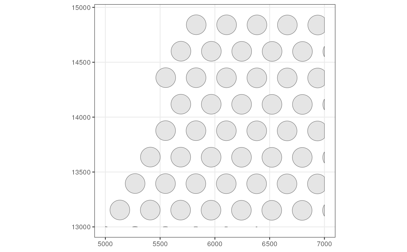
#> AGTGAGCCTCGCCGCC POLYGON ((5222.552 13154.04... Vis5AHere we get a sf data frame, which is just like a
regular data frame but with a special geometry column. Now
plot these spot polygons
# Set colGeometry
colGeometry(sfe_tissue, "spotPoly") <- spots
To see which colGeometries are present in the SFE
object:
colGeometryNames(sfe_tissue)
#> [1] "spotPoly"
There are shorthands for some specific column or row geometries. For
example, spotPoly(sfe) is equivalent to
colGeometry(sfe, "spotPoly") shown above.
# Getter
(spots <- spotPoly(sfe_tissue))
#> Simple feature collection with 57 features and 1 field
#> Geometry type: POLYGON
#> Dimension:     XY
#> Bounding box:  xmin: 5000 ymin: 13000 xmax: 7000 ymax: 14931.74
#> CRS:           NA
#> First 10 features:
#>                                        geometry sample_id
#> AAATTACCTATCGATG POLYGON ((6472.186 13875.23...     Vis5A
#> AACATATCAACTGGTG POLYGON ((5778.291 13635.43...     Vis5A
#> AAGATTGGCGGAACGT POLYGON ((7000 13809.84, 69...     Vis5A
#> AAGGGACAGATTCTGT POLYGON ((6749.535 13874.64...     Vis5A
#> AATATCGAGGGTTCTC POLYGON ((5500.941 13636.03...     Vis5A
#> AATGATGATACGCTAT POLYGON ((6612.42 14598.82,...     Vis5A
#> AATTCATAAGGGATCT POLYGON ((6889.769 14598.22...     Vis5A
#> ACGCTAGTGATACACT POLYGON ((5639.096 13394.44...     Vis5A
#> AGCGCGGGTGCCAATG POLYGON ((6750.575 14357.23...     Vis5A
#> AGTGAGCCTCGCCGCC POLYGON ((5222.552 13154.04...     Vis5A
# Setter
spotPoly(sfe_tissue) <- spots
Exercise: The cellSeg function gets cell segmentation
from the MERFISH dataset in sfe_vizgen. Get and plot the
cell segmentations.
Annotation
Annotation geometries can be get or set with
annotGeometry(). In column or row geometries, the number of
rows of the sf data frame (i.e. the number of geometries in
the data frame) is constrained by the number of rows or columns of the
gene count matrix respectively, because just like rowData
and colData, each row of a rowGeometry or
colGeometry sf data frame must correspond to a
row or column of the gene count matrix respectively. In contrast, an
annotGeometry sf data frame can have any
dimension, not constrained by the dimension of the gene count
matrix.
# Getter, by name or index
(tb <- annotGeometry(sfe_tissue, "tissueBoundary"))
#> Simple feature collection with 1 feature and 2 fields
#> Geometry type: POLYGON
#> Dimension:     XY
#> Bounding box:  xmin: 5094 ymin: 13000 xmax: 7000 ymax: 14969
#> CRS:           NA
#>   ID                       geometry sample_id
#> 7  7 POLYGON ((5094 13000, 5095 ...     Vis5A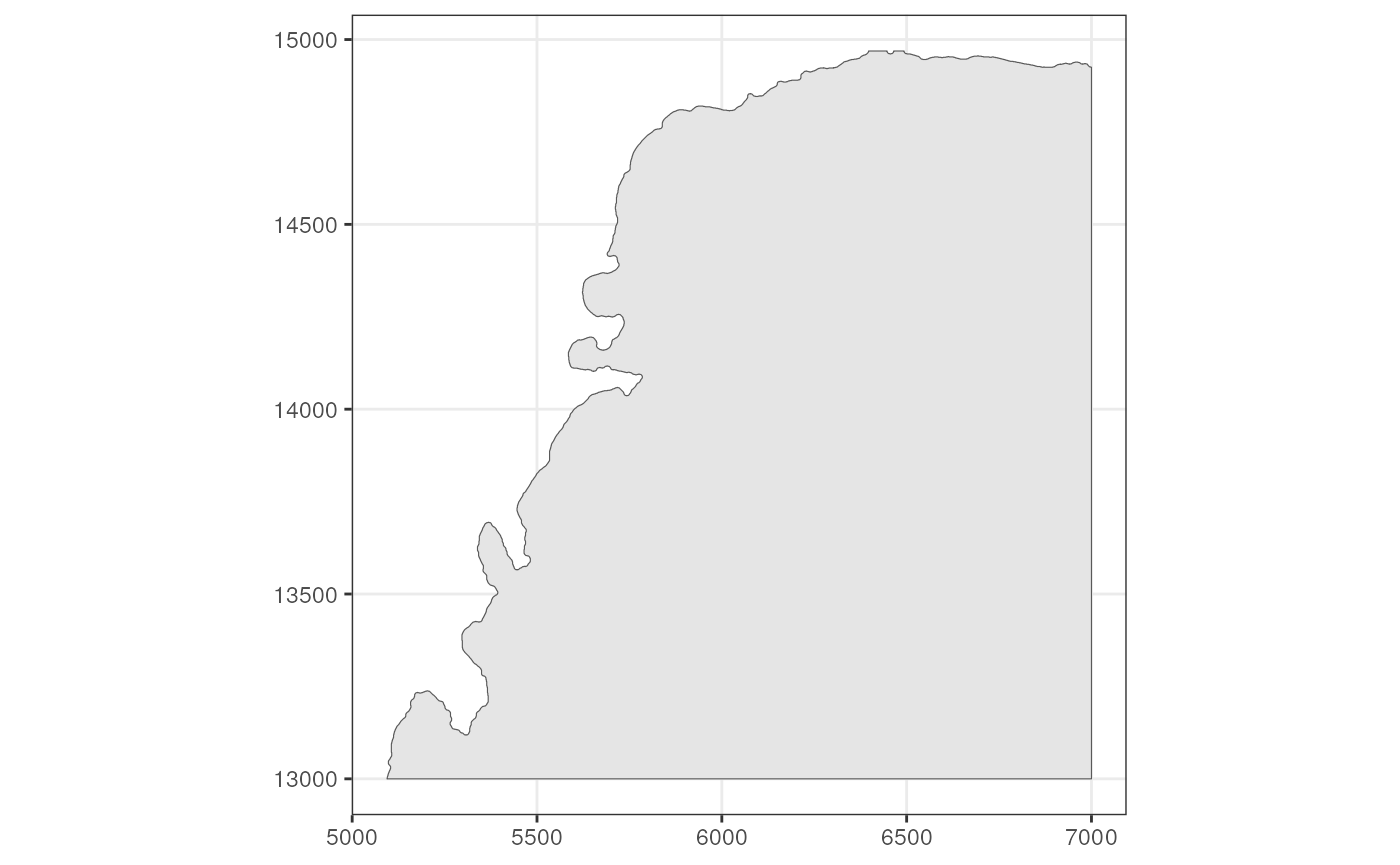
# Setter, by name or index
annotGeometry(sfe_tissue, "tissueBoundary") <- tb
See which annotGeometries are present in the SFE
object:
annotGeometryNames(sfe_tissue)
#> [1] "tissueBoundary"      "myofiber_full"       "myofiber_simplified"
#> [4] "nuclei"              "nuclei_centroid"
There are shorthands for specific annotation geometries. For example,
tissueBoundary(sfe) is equivalent to
annotGeometry(sfe, "tissueBoundary").
cellSeg() (cell segmentation) and nucSeg()
(nuclei segmentation) would first query colGeometries (for
single cell, single molecule technologies, equivalent to
colGeometry(sfe, "cellSeg") or
colGeometry(sfe, "nucSeg")), and if not found, they will
query annotGeometries (for array capture and
microdissection technologies, equivalent to
annotGeometry(sfe, "cellSeg") or
annotGeometry(sfe, "nucSeg")).
# Getter
(tb <- tissueBoundary(sfe_tissue))
#> Simple feature collection with 1 feature and 2 fields
#> Geometry type: POLYGON
#> Dimension:     XY
#> Bounding box:  xmin: 5094 ymin: 13000 xmax: 7000 ymax: 14969
#> CRS:           NA
#>   ID                       geometry sample_id
#> 7  7 POLYGON ((5094 13000, 5095 ...     Vis5A
# Setter
tissueBoundary(sfe_tissue) <- tb
Spatial graphs
The spatial neighborhood graphs for Visium spots are stored in the
colGraphs field, which has similar user interface as
colGeometries. SFE also wraps all methods to find the
spatial neighborhood graph implemented in the spdep
package, and triangulation is used here as demonstration.
(g <- findSpatialNeighbors(sfe_tissue, MARGIN = 2, method = "tri2nb"))
#> Characteristics of weights list object:
#> Neighbour list object:
#> Number of regions: 57
#> Number of nonzero links: 314
#> Percentage nonzero weights: 9.664512
#> Average number of links: 5.508772
#>
#> Weights style: W
#> Weights constants summary:
#>    n   nn S0       S1       S2
#> W 57 3249 57 20.93315 229.9213
plot(g, coords = spatialCoords(sfe_tissue))
# Set graph by name
colGraph(sfe_tissue, "graph1") <- g
# Get graph by name
(g <- colGraph(sfe_tissue, "graph1"))
#> Characteristics of weights list object:
#> Neighbour list object:
#> Number of regions: 57
#> Number of nonzero links: 314
#> Percentage nonzero weights: 9.664512
#> Average number of links: 5.508772
#>
#> Weights style: W
#> Weights constants summary:
#>    n   nn S0       S1       S2
#> W 57 3249 57 20.93315 229.9213
For Visium, spatial neighborhood graph of the hexagonal grid can be
found with the known locations of the barcodes. One SFE object can have
multiple colGraphs.
colGraph(sfe_tissue, "visium") <- findVisiumGraph(sfe_tissue)
plot(colGraph(sfe_tissue, "visium"), coords = spatialCoords(sfe_tissue))
Which graphs are present in this SFE object?
colGraphNames(sfe_tissue)
#> [1] "graph1" "visium"
While this workshop only works with one sample, i.e. tissue section, operations on multiple samples is discussed in the vignette of the SFE package.
Row geometries
The Visium dataset does not have geometries associated with genes,
but the MERFISH dataset does. The rowGeometry getter and
setter have pretty much the same user interface as the getters and
setters covered above:
(rg <- rowGeometry(sfe_vizgen, "txSpots"))
#> Simple feature collection with 62 features and 4 fields
#> Geometry type: MULTIPOINT
#> Dimension:     XY
#> Bounding box:  xmin: 6500.184 ymin: -1499.778 xmax: 6799.719 ymax: -1200.041
#> CRS:           NA
#> First 10 features:
#>          gene barcode_id global_z   transcript_id
#> CD4       CD4          0        3 ENST00000011653
#> TLL1     TLL1          1        3 ENST00000061240
#> EPHA8   EPHA8          2        3 ENST00000166244
#> CDKN1A CDKN1A          4        3 ENST00000244741
#> PDGFRA PDGFRA          6        3 ENST00000257290
#> CD44     CD44          7        3 ENST00000263398
#> FCGR2A FCGR2A          8        3 ENST00000271450
#> EGFR     EGFR          9        3 ENST00000275493
#> DRAXIN DRAXIN         11        3 ENST00000294485
#> LMX1A   LMX1A         12        3 ENST00000294816
#>                              geometry
#> CD4    MULTIPOINT ((6770.52 -1466....
#> TLL1   MULTIPOINT ((6692.258 -1435...
#> EPHA8  MULTIPOINT ((6531.73 -1427....
#> CDKN1A MULTIPOINT ((6774.421 -1477...
#> PDGFRA MULTIPOINT ((6642.847 -1355...
#> CD44   MULTIPOINT ((6530.448 -1449...
#> FCGR2A MULTIPOINT ((6589.974 -1481...
#> EGFR   MULTIPOINT ((6655.547 -1419...
#> DRAXIN MULTIPOINT ((6708.042 -1317...
#> LMX1A  MULTIPOINT ((6797.345 -1240...
# Setter
rowGeometry(sfe_vizgen, "txSpots") <- rg
In the case of transcript spots, there’s a special convenience
function txSpots
txSpots(sfe_vizgen)
#> Simple feature collection with 62 features and 4 fields
#> Geometry type: MULTIPOINT
#> Dimension:     XY
#> Bounding box:  xmin: 6500.184 ymin: -1499.778 xmax: 6799.719 ymax: -1200.041
#> CRS:           NA
#> First 10 features:
#>          gene barcode_id global_z   transcript_id
#> CD4       CD4          0        3 ENST00000011653
#> TLL1     TLL1          1        3 ENST00000061240
#> EPHA8   EPHA8          2        3 ENST00000166244
#> CDKN1A CDKN1A          4        3 ENST00000244741
#> PDGFRA PDGFRA          6        3 ENST00000257290
#> CD44     CD44          7        3 ENST00000263398
#> FCGR2A FCGR2A          8        3 ENST00000271450
#> EGFR     EGFR          9        3 ENST00000275493
#> DRAXIN DRAXIN         11        3 ENST00000294485
#> LMX1A   LMX1A         12        3 ENST00000294816
#>                              geometry
#> CD4    MULTIPOINT ((6770.52 -1466....
#> TLL1   MULTIPOINT ((6692.258 -1435...
#> EPHA8  MULTIPOINT ((6531.73 -1427....
#> CDKN1A MULTIPOINT ((6774.421 -1477...
#> PDGFRA MULTIPOINT ((6642.847 -1355...
#> CD44   MULTIPOINT ((6530.448 -1449...
#> FCGR2A MULTIPOINT ((6589.974 -1481...
#> EGFR   MULTIPOINT ((6655.547 -1419...
#> DRAXIN MULTIPOINT ((6708.042 -1317...
#> LMX1A  MULTIPOINT ((6797.345 -1240...
Plot the transcript spots (for the toy dataset, they were subsampled to keep the SFE package small; usually they are much denser)
Images
In SPE, the images are only used for visualization, but SFE extended the SPE image functionality so large images don’t have to be loaded into memory unless necessary. In SFE, there are 3 types of images:
-
SpatRasterImage, the default, a thin wrapper around theSpatRasterclass in theterraobject to make it conform to SPE’s requirements. Large images are not loaded into memory unless necessary and it’s possible to only load a down sampled lower resolution version of the image into memory. Spatial extent is part ofSpatRaster. The extent is important to delineate where the image is in the coordinate system within the tissue section. This is a more sophisticated way to make sure the image is aligned with the geometries than the scale factor in SPE which only works for Visium and would not allow the SPE object to be cropped. -
BioFormatsImageis used forOME-TIFFimages whose compression can’t be read byterra. The image is not loaded into memory. It’s just some metadata, which includes the file path, extent, and origin (minimum value of coordinates). So far functions related toBioFormatsImagecater to Xenium data. -
EBImageis a thin wrapper around theImageclass in theEBImagepackage to conform to SPE’s requirements. WithEBImage, one can do thresholding and morphological operations. However, it’s not merely a wrapper; it contains another metadata field for the extent. WhenBioFormatsImageis loaded into memory, it becomesEBImage.
In the MERFISH dataset above, the image is represented as
SpatRasterImage. Get images with the getImg
function, and use the image_id function to indicate which
image to get, and if it’s left blank, the first imaget will be
retrieved:
(img <- getImg(sfe_vizgen, image_id = "DAPI_z3"))
#> 1 x 695 x 695 (width x height) SpatRasterImage
#> imgSource():
#>   /__w/VoyagerHackathon/VoyagerHackathon/vignettes/vizgen_cellbound/images/mosaic_
#>   DAPI_z3.tif
Use th ext function to get the extent of the image
ext(img)
#>      xmin      xmax      ymin      ymax
#>  6499.909  6800.141 -1500.166 -1199.939
SpatRasterImage is a thin wrapper; use
imgRaster to get the image itself:
plot(imgRaster(img), col = viridis_pal()(50))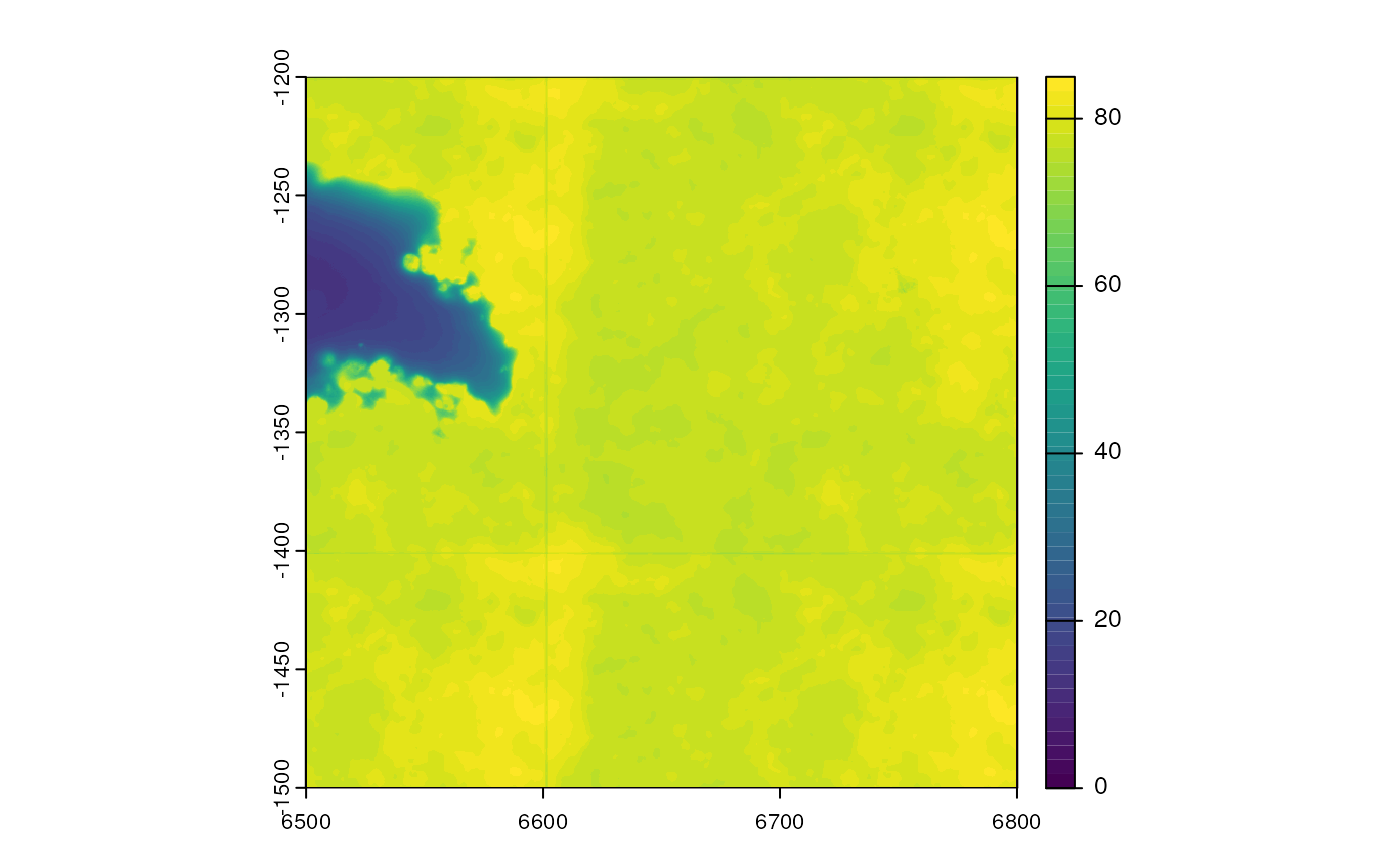
The advantage of SpatRasterImage is that one can use
vector geometries such as in sf data frames to extract data
from the raster image. With a binary mask, the terra
package can convert the mask into polygons and vice versa.
But there are some disadvantages, such as that terra is
built for geography so it’s difficult to perform affine transforms of
the image (including rotation); in geography the transformation is
performed by reprojecting the map and there are standards for the
projections such as the Mercator and Robinson projections of the world
map. So when the SpatRasterImage is rotated, it’s converted
into EBImage, which can be converted back to
SpatRasterImage. BioFormatsImage can also be
converted into SpatRasterImage though that goes through
EBImage. Also, one cannot perform image processing such as
morphological operations, watershed segmentation, and so on that can be
performed by EBImage.
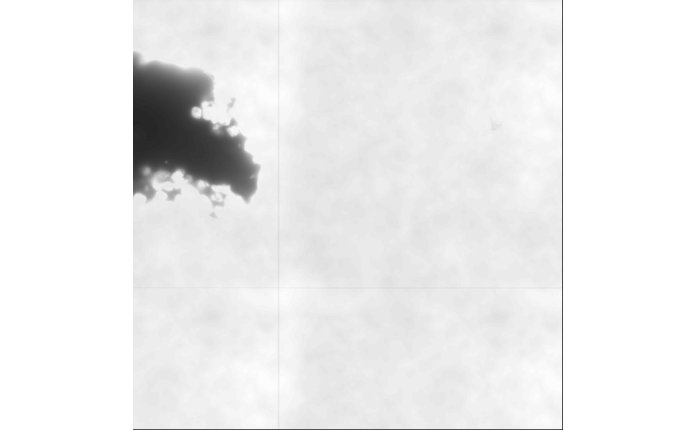
Here we convert this image into EBImage, and plot it
with the EBImage package
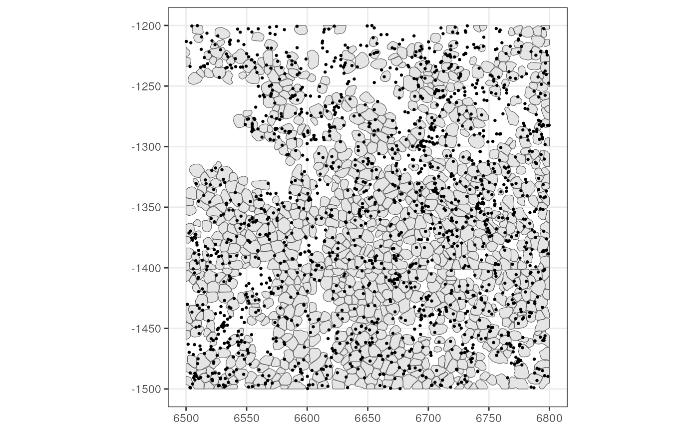
Finally, we can call a Voyager function to plot the image, cell segmentation, and transcript spots together:
plotSpatialFeature(sfe_vizgen, features = "volume", colGeometryName = "cellSeg",
                   image_id = "DAPI_z3", dark = TRUE) +
    geom_sf(data = rg, size = 0.1, color = "white")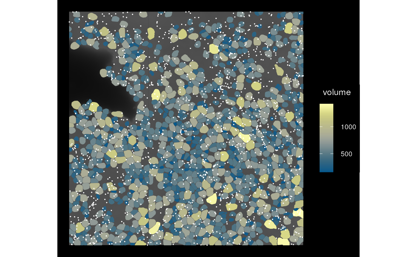
BTW, the reason why the transcript spots are not assigned to cells
but stored in rowGeometries as MULTIPOINT is
that some transcript spots are not in any segmented cells as shown in
this plot. However, it doesn’t mean that they are irrelevant.
Also, the plot above shows transcript spots from all genes in this
dataset and they’re very down sampled. In the hackathon, you may choose
to work on this issue to
add rowGeometries to the plotSpatialFeature
function and add an argument to specify which gene(s) to plot. Typically
only a small number of genes should be plotted at a time, because
otherwise the points will be too crowded to see and if using colors to
distinguish between genes, there will be colors that are difficult to
distinguish. I suggest using point shape to distinguish between genes
when colors are already used for cell data.
Turn the above code chunk into a function as we’ll call it several times more though only for this MERFISH dataset
plot_sfe_vizgen <- function(sfe) {
    plotSpatialFeature(sfe, features = "volume", colGeometryName = "cellSeg",
                   image_id = "DAPI_z3", dark = TRUE) +
    geom_sf(data = txSpots(sfe), size = 0.1, color = "white")
}
Spatial operations
Bounding box
The bounding box of a geometry is the smallest rectangle that
contains this geometry, so you get minimum and maximum x coordinates and
y coordinates. We can find the bounding box of individual
sf data frames with st_bbox from the
sf package
st_bbox(rg)
#>      xmin      ymin      xmax      ymax
#>  6500.184 -1499.778  6799.719 -1200.041
However, in an SFE object, there are multiple geometries, such as
cell centroids, cell segmentation, nucleus segmentation, tissue
boundary, transcript spots, and so on, and there are images. The
bbox function for SFE aggregates the bounding boxes of all
the geometries (and optionally images) to get an overall bounding box of
the SFE object:
bbox(sfe_vizgen)
#>      xmin      ymin      xmax      ymax
#>  6498.553 -1502.179  6800.404 -1199.928
# In this case the image is not larger than the geometries
bbox(sfe_vizgen, include_image = TRUE)
#>      xmin      ymin      xmax      ymax
#>  6498.553 -1502.179  6800.404 -1199.928
Cropping
You can think of the SFE object as a stack of maps that are aligned,
like the National Map
layers of satellite images, land use, administrative boundaries,
watersheds, rock formations, faults, and etc. Cropping will crop all of
the maps. One can crop with either a bounding box or a polygon of any
shape. The colGeometryName argument specifies the
colGeometry to decide which cell to keep after cropping.
Using the centroid would be different from using the cell polygon since
a polygon can slightly overlap with the bounding box while the centroid
is outside.
bbox_use <- c(xmin = 6550, xmax = 6650, ymin = -1350, ymax = -1250)
sfe_cropped <- crop(sfe_vizgen, bbox_use, colGeometryName = "cellSeg")
bbox(sfe_cropped)
#>  xmin  ymin  xmax  ymax
#>  6550 -1350  6650 -1250
plot_sfe_vizgen(sfe_cropped)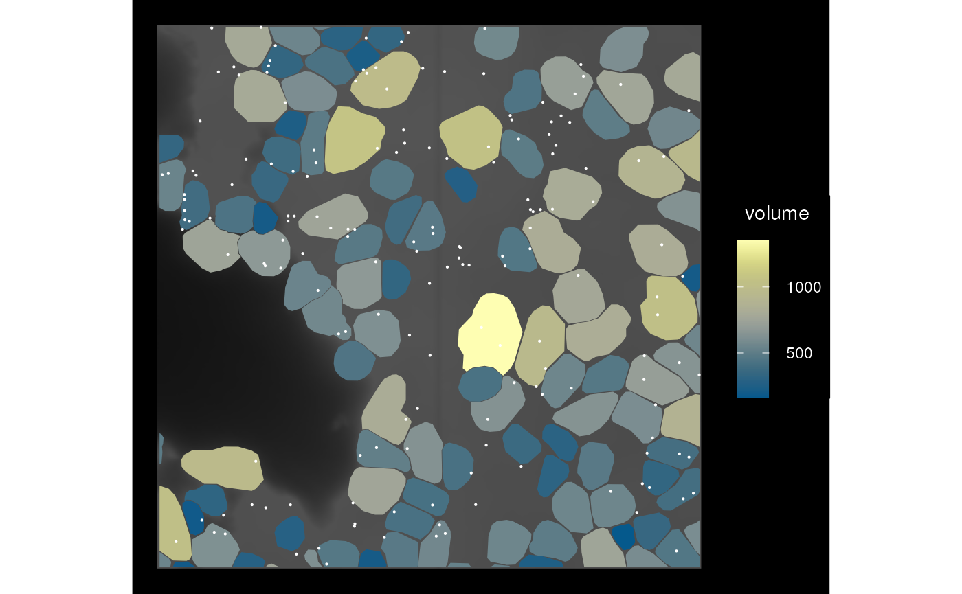
Don’t like those tiny slivers of cells at the boundary of the
bounding box? We can also keep any cell that intersects with the
bounding box and with larger datasets, this is much faster than finding
the actual intersection geometries. The keep_whole argument
makes sure that the cells are kept whole; “col” because it can also be
“annot” to keep annotGeometry items (e.g. cell segmentation
in Visium datasets) whole.
sfe_cropped2 <- crop(sfe_vizgen, bbox_use, colGeometryName = "cellSeg",
                     keep_whole = "col")
plot_sfe_vizgen(sfe_cropped2) +
    geom_sf(data = st_as_sfc(st_bbox(bbox_use)), fill = NA, color = "red",
            linewidth = 0.5)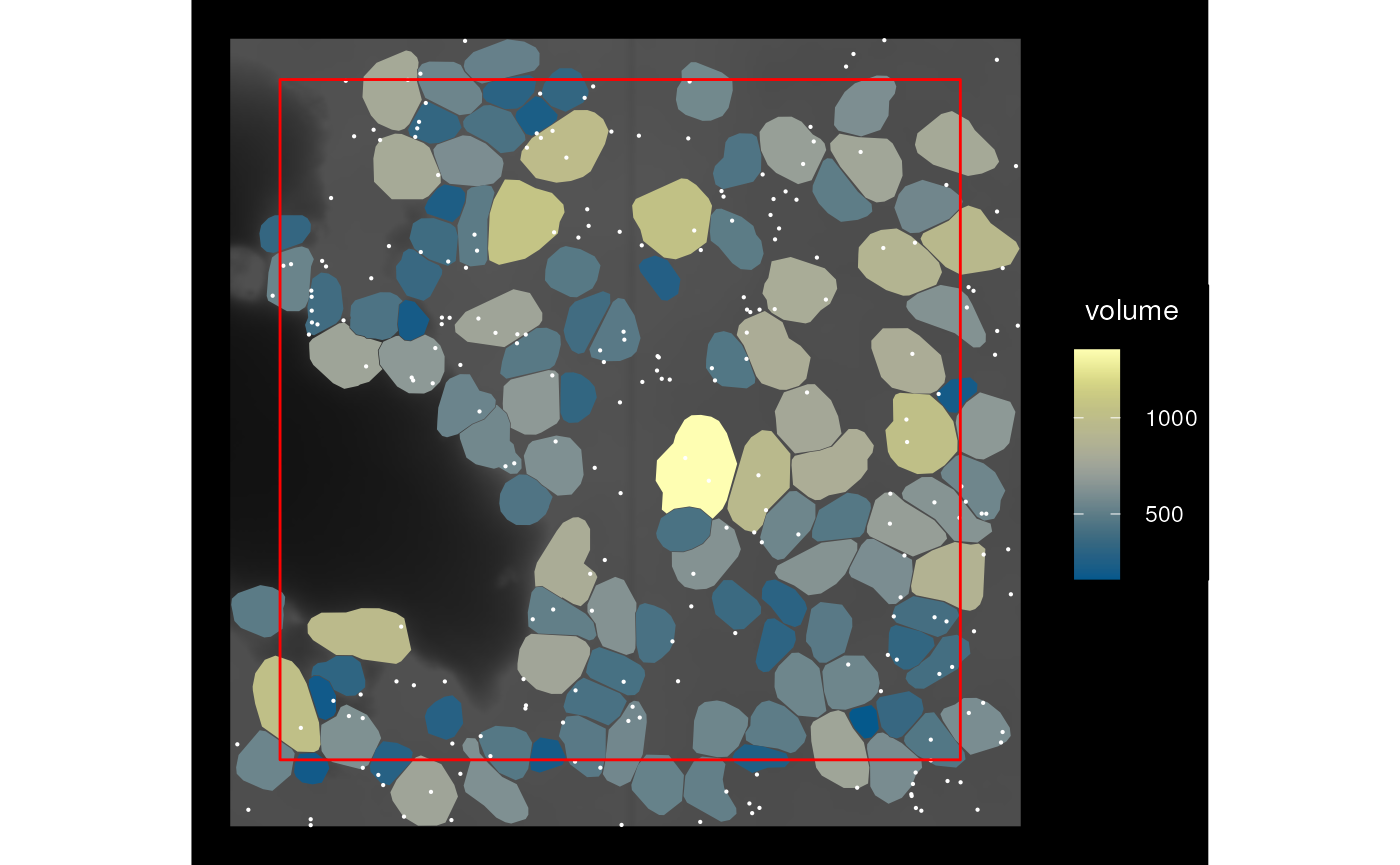
Here the original bounding box is shown in red and the cells that partially overlap are not cropped.
We can also only keep cells covered by (i.e. entirely within) the bounding box
sfe_cropped3 <- crop(sfe_vizgen, bbox_use, colGeometryName = "cellSeg",
                     keep_whole = "col", cover = TRUE)
plot_sfe_vizgen(sfe_cropped3)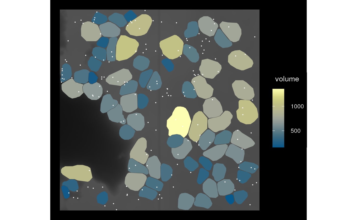
We can also use a geometry to remove a part of the data by specifying
op = st_difference; keep_whole and
cover still apply.
sfe_hole <- crop(sfe_vizgen, bbox_use, colGeometryName = "cellSeg",
                 op = st_difference)
plot_sfe_vizgen(sfe_hole)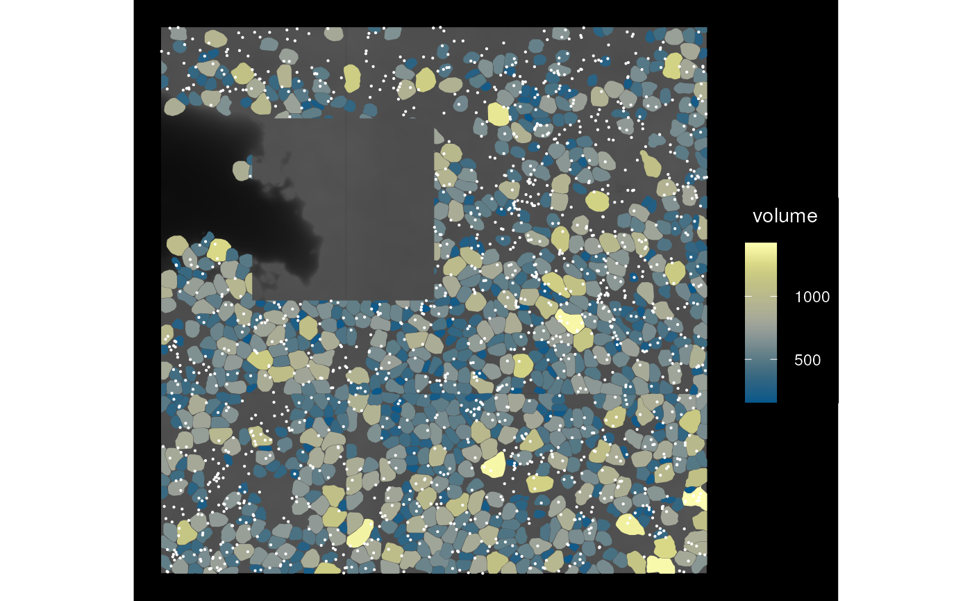
Transformation
We can rotate (right now only multiples of 90 degrees), mirror, transpose, and translate the SFE object, such as when there’s a canonical orientation like in brain sections but the data is of a different orientation when read in. Here all geometries and images are transformed while keeping them aligned.
sfe_mirror <- mirror(sfe_vizgen, direction = "vertical")
plot_sfe_vizgen(sfe_mirror)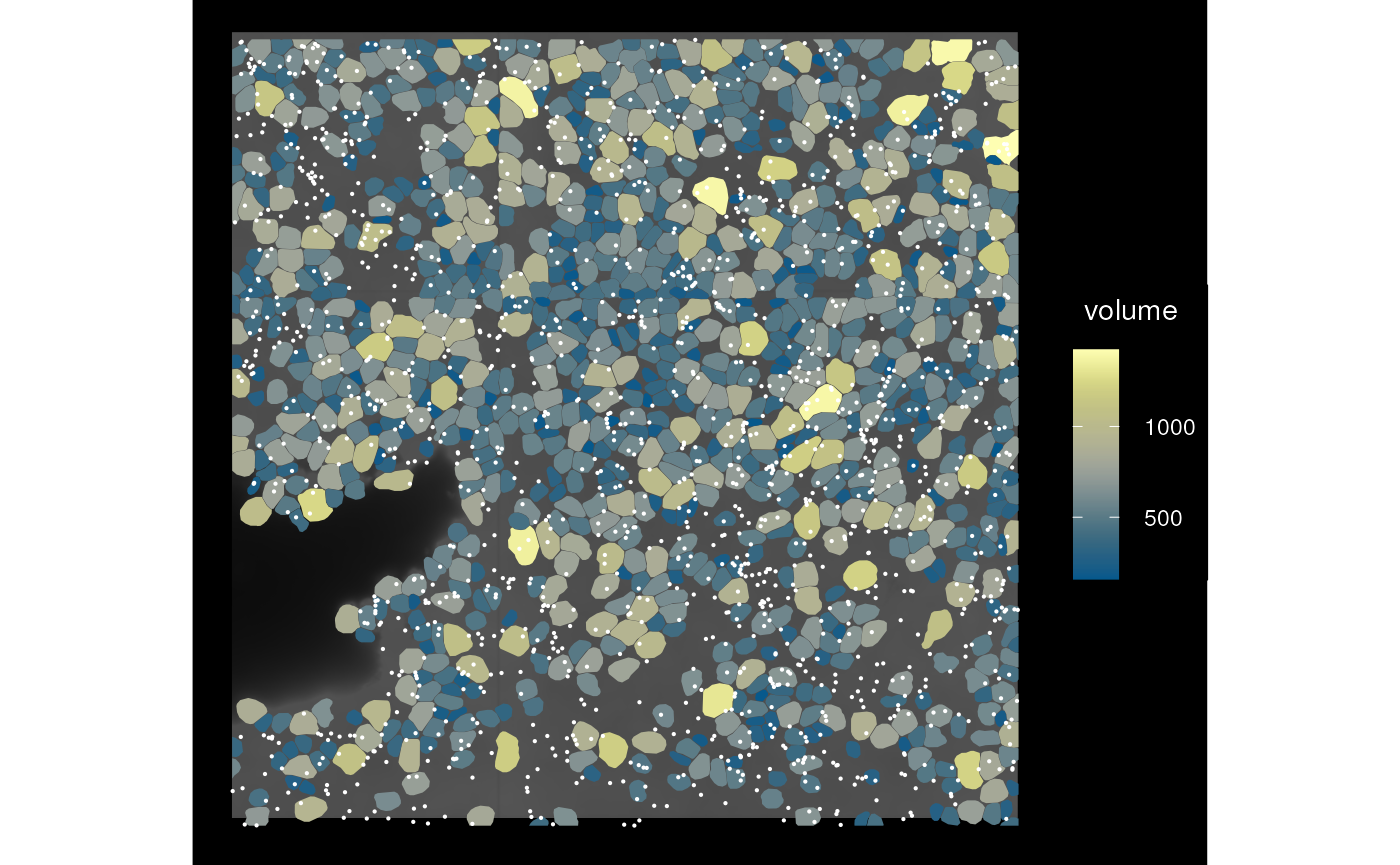
Individual images can be transformed say in case it doesn’t initially align with the geometries, though for this dataset, this will put the image out of alignment
sfe_img <- mirrorImg(sfe_vizgen, image_id = "DAPI_z3")
plot_sfe_vizgen(sfe_img)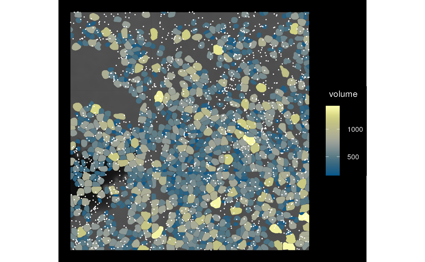
Multiple samples
Thus far, the example dataset used only has one sample. The
SpatialExperiment (SPE) object has a special column in
colData called sample_id, so data from
multiple tissue sections can coexist in the same SPE object for joint
dimension reduction and clustering while keeping the spatial coordinates
separate. It’s important to keep spatial coordinates of different tissue
sections separate because first, the coordinates would only make sense
within the same section, and second, the coordinates from different
sections can have overlapping numeric values.
SFE inherits from SPE, and with geometries and spatial graphs,
sample_id is even more important. The geometry and graph
getter and setter functions have a sample_id argument,
which is optional when only one sample is present in the SFE object.
This argument is mandatory if multiple samples are present, and can be a
character vector for multiple samples or “all” for all samples. Below
are examples of using the getters and setters for multiple samples.
# Construct toy dataset with 2 samples
sfe1 <- McKellarMuscleData(dataset = "small")
#> see ?SFEData and browseVignettes('SFEData') for documentation
#> loading from cache
sfe2 <- McKellarMuscleData(dataset = "small2")
#> see ?SFEData and browseVignettes('SFEData') for documentation
#> loading from cache
spotPoly(sfe2)$sample_id <- "sample02"
(sfe_combined <- cbind(sfe1, sfe2))
#> class: SpatialFeatureExperiment
#> dim: 15123 149
#> metadata(0):
#> assays(1): counts
#> rownames(15123): ENSMUSG00000025902 ENSMUSG00000096126 ...
#>   ENSMUSG00000064368 ENSMUSG00000064370
#> rowData names(6): Ensembl symbol ... vars cv2
#> colnames(149): AAATTACCTATCGATG AACATATCAACTGGTG ... TTCCTCGGACTAACCA
#>   TTCTGACCGGGCTCAA
#> colData names(12): barcode col ... prop_mito in_tissue
#> reducedDimNames(0):
#> mainExpName: NULL
#> altExpNames(0):
#> spatialCoords names(2) : imageX imageY
#> imgData names(1): sample_id
#>
#> unit: full_res_image_pixels
#> Geometries:
#> colGeometries: spotPoly (POLYGON)
#> annotGeometries: tissueBoundary (GEOMETRY), myofiber_full (GEOMETRY), myofiber_simplified (GEOMETRY), nuclei (POLYGON), nuclei_centroid (POINT)
#>
#> Graphs:
#> Vis5A:
#> sample02:
Use the sampleIDs function to see the names of all
samples
sampleIDs(sfe_combined)
#> [1] "Vis5A"    "sample02"
# Only get the geometries for the second sample
(spots2 <- colGeometry(sfe_combined, "spotPoly", sample_id = "sample02"))
#> Simple feature collection with 72 features and 1 field
#> Geometry type: POLYGON
#> Dimension:     XY
#> Bounding box:  xmin: 6000 ymin: 7025.865 xmax: 8000 ymax: 9000
#> CRS:           NA
#> First 10 features:
#>                  sample_id                       geometry
#> AACACACGCTCGCCGC  sample02 POLYGON ((6597.869 7842.575...
#> AACCGCTAAGGGATGC  sample02 POLYGON ((6724.811 9000, 67...
#> AACGCTGTTGCTGAAA  sample02 POLYGON ((6457.635 7118.991...
#> AACGGACGTACGTATA  sample02 POLYGON ((6737.064 8083.571...
#> AATAGAATCTGTTTCA  sample02 POLYGON ((7570.153 8564.368...
#> ACAAATCGCACCGAAT  sample02 POLYGON ((8000 7997.001, 79...
#> ACAATTGTGTCTCTTT  sample02 POLYGON ((6043.169 7843.77,...
#> ACAGGCTTGCCCGACT  sample02 POLYGON ((7428.88 7358.195,...
#> ACCAGTGCGGGAGACG  sample02 POLYGON ((6460.753 8566.757...
#> ACCCTCCCTTGCTATT  sample02 POLYGON ((7847.503 8563.771...
# Only set the geometries for the second sample
# Leaving geometries of the first sample intact
colGeometry(sfe_combined, "spotPoly", sample_id = "sample02") <- spots2
# Set graph only for the second sample
colGraph(sfe_combined, "foo", sample_id = "sample02") <-
  findSpatialNeighbors(sfe_combined, sample_id = "sample02")
# Get graph only for the second sample
colGraph(sfe_combined, "foo", sample_id = "sample02")
#> Characteristics of weights list object:
#> Neighbour list object:
#> Number of regions: 72
#> Number of nonzero links: 406
#> Percentage nonzero weights: 7.83179
#> Average number of links: 5.638889
#>
#> Weights style: W
#> Weights constants summary:
#>    n   nn S0       S1       S2
#> W 72 5184 72 25.82104 289.8299
# Set graph of the same name for both samples
# The graphs are computed separately for each sample
colGraphs(sfe_combined, sample_id = "all", name = "visium") <-
  findVisiumGraph(sfe_combined, sample_id = "all")
# Get multiple graphs of the same name
colGraphs(sfe_combined, sample_id = "all", name = "visium")
#> $Vis5A
#> Characteristics of weights list object:
#> Neighbour list object:
#> Number of regions: 77
#> Number of nonzero links: 394
#> Percentage nonzero weights: 6.645303
#> Average number of links: 5.116883
#>
#> Weights style: W
#> Weights constants summary:
#>    n   nn S0       S1       S2
#> W 77 5929 77 31.68056 311.7544
#>
#> $sample02
#> Characteristics of weights list object:
#> Neighbour list object:
#> Number of regions: 72
#> Number of nonzero links: 366
#> Percentage nonzero weights: 7.060185
#> Average number of links: 5.083333
#>
#> Weights style: W
#> Weights constants summary:
#>    n   nn S0       S1       S2
#> W 72 5184 72 29.83889 291.5833
# Or just all graphs of the margin
colGraphs(sfe_combined, sample_id = "all")
#> $Vis5A
#> $Vis5A$visium
#> Characteristics of weights list object:
#> Neighbour list object:
#> Number of regions: 77
#> Number of nonzero links: 394
#> Percentage nonzero weights: 6.645303
#> Average number of links: 5.116883
#>
#> Weights style: W
#> Weights constants summary:
#>    n   nn S0       S1       S2
#> W 77 5929 77 31.68056 311.7544
#>
#>
#> $sample02
#> $sample02$foo
#> Characteristics of weights list object:
#> Neighbour list object:
#> Number of regions: 72
#> Number of nonzero links: 406
#> Percentage nonzero weights: 7.83179
#> Average number of links: 5.638889
#>
#> Weights style: W
#> Weights constants summary:
#>    n   nn S0       S1       S2
#> W 72 5184 72 25.82104 289.8299
#>
#> $sample02$visium
#> Characteristics of weights list object:
#> Neighbour list object:
#> Number of regions: 72
#> Number of nonzero links: 366
#> Percentage nonzero weights: 7.060185
#> Average number of links: 5.083333
#>
#> Weights style: W
#> Weights constants summary:
#>    n   nn S0       S1       S2
#> W 72 5184 72 29.83889 291.5833
Sample IDs can also be changed, with the
changeSampleIDs() function, with a named vector whose names
are the old names and values are the new names.
sfe_combined <- changeSampleIDs(sfe_combined,
                                replacement = c(Vis5A = "foo", sample02 = "bar"))
sfe_combined
#> class: SpatialFeatureExperiment
#> dim: 15123 149
#> metadata(0):
#> assays(1): counts
#> rownames(15123): ENSMUSG00000025902 ENSMUSG00000096126 ...
#>   ENSMUSG00000064368 ENSMUSG00000064370
#> rowData names(6): Ensembl symbol ... vars cv2
#> colnames(149): AAATTACCTATCGATG AACATATCAACTGGTG ... TTCCTCGGACTAACCA
#>   TTCTGACCGGGCTCAA
#> colData names(12): barcode col ... prop_mito in_tissue
#> reducedDimNames(0):
#> mainExpName: NULL
#> altExpNames(0):
#> spatialCoords names(2) : imageX imageY
#> imgData names(1): sample_id
#>
#> unit: full_res_image_pixels
#> Geometries:
#> colGeometries: spotPoly (POLYGON)
#> annotGeometries: tissueBoundary (GEOMETRY), myofiber_full (GEOMETRY), myofiber_simplified (GEOMETRY), nuclei (POLYGON), nuclei_centroid (POINT)
#>
#> Graphs:
#> foo: col: visium
#> bar: col: foo, visium
Basically, all the functions covered above have an argument
sample_id if the operation is not to be performed on all
samples. Or set sample_id = "all" to perform on all
samples.
sampleIDs(sfe_combined)
#> [1] "foo" "bar"
bbox(sfe_combined, sample_id = "all")
#>        foo  bar
#> xmin  5000 6000
#> ymin 13000 7000
#> xmax  7000 8000
#> ymax 15000 9000
bbox(sfe_combined, sample_id = "foo")
#>  xmin  ymin  xmax  ymax
#>  5000 13000  7000 15000
Future directions
See the GitHub issues
Session info
sessionInfo()
#> R Under development (unstable) (2024-02-28 r85999)
#> Platform: x86_64-pc-linux-gnu
#> Running under: Ubuntu 22.04.3 LTS
#>
#> Matrix products: default
#> BLAS:   /usr/lib/x86_64-linux-gnu/openblas-pthread/libblas.so.3
#> LAPACK: /usr/lib/x86_64-linux-gnu/openblas-pthread/libopenblasp-r0.3.20.so;  LAPACK version 3.10.0
#>
#> locale:
#>  [1] LC_CTYPE=en_US.UTF-8       LC_NUMERIC=C
#>  [3] LC_TIME=en_US.UTF-8        LC_COLLATE=en_US.UTF-8
#>  [5] LC_MONETARY=en_US.UTF-8    LC_MESSAGES=en_US.UTF-8
#>  [7] LC_PAPER=en_US.UTF-8       LC_NAME=C
#>  [9] LC_ADDRESS=C               LC_TELEPHONE=C
#> [11] LC_MEASUREMENT=en_US.UTF-8 LC_IDENTIFICATION=C
#>
#> time zone: Etc/UTC
#> tzcode source: system (glibc)
#>
#> attached base packages:
#> [1] stats4    stats     graphics  grDevices utils     datasets  methods
#> [8] base
#>
#> other attached packages:
#>  [1] scales_1.3.0                   EBImage_4.45.0
#>  [3] Voyager_1.5.0                  SFEData_1.5.0
#>  [5] SpatialFeatureExperiment_1.5.2 scran_1.31.0
#>  [7] scater_1.31.2                  scuttle_1.13.0
#>  [9] SingleCellExperiment_1.25.0    SummarizedExperiment_1.33.3
#> [11] Biobase_2.63.0                 GenomicRanges_1.55.3
#> [13] GenomeInfoDb_1.39.6            IRanges_2.37.1
#> [15] S4Vectors_0.41.3               BiocGenerics_0.49.1
#> [17] MatrixGenerics_1.15.0          matrixStats_1.2.0
#> [19] ggplot2_3.5.0                  terra_1.7-71
#> [21] sf_1.0-15                      BiocStyle_2.31.0
#>
#> loaded via a namespace (and not attached):
#>   [1] bitops_1.0-7              filelock_1.0.3
#>   [3] tibble_3.2.1              R.oo_1.26.0
#>   [5] lifecycle_1.0.4           edgeR_4.1.17
#>   [7] lattice_0.22-5            magrittr_2.0.3
#>   [9] limma_3.59.3              sass_0.4.8
#>  [11] rmarkdown_2.25            jquerylib_0.1.4
#>  [13] yaml_2.3.8                metapod_1.11.1
#>  [15] sp_2.1-3                  DBI_1.2.2
#>  [17] abind_1.4-5               zlibbioc_1.49.0
#>  [19] purrr_1.0.2               R.utils_2.12.3
#>  [21] RCurl_1.98-1.14           rappdirs_0.3.3
#>  [23] GenomeInfoDbData_1.2.11   ggrepel_0.9.5
#>  [25] irlba_2.3.5.1             units_0.8-5
#>  [27] RSpectra_0.16-1           dqrng_0.3.2
#>  [29] pkgdown_2.0.7             DelayedMatrixStats_1.25.1
#>  [31] codetools_0.2-19          DropletUtils_1.23.0
#>  [33] DelayedArray_0.29.8       tidyselect_1.2.0
#>  [35] farver_2.1.1              ScaledMatrix_1.11.0
#>  [37] viridis_0.6.5             BiocFileCache_2.11.1
#>  [39] jsonlite_1.8.8            BiocNeighbors_1.21.2
#>  [41] e1071_1.7-14              systemfonts_1.0.5
#>  [43] ggnewscale_0.4.10         tools_4.4.0
#>  [45] ragg_1.2.7                sfarrow_0.4.1
#>  [47] Rcpp_1.0.12               glue_1.7.0
#>  [49] gridExtra_2.3             SparseArray_1.3.4
#>  [51] xfun_0.42                 dplyr_1.1.4
#>  [53] HDF5Array_1.31.6          withr_3.0.0
#>  [55] BiocManager_1.30.22       fastmap_1.1.1
#>  [57] boot_1.3-30               rhdf5filters_1.15.2
#>  [59] bluster_1.13.0            fansi_1.0.6
#>  [61] spData_2.3.0              digest_0.6.34
#>  [63] rsvd_1.0.5                mime_0.12
#>  [65] R6_2.5.1                  textshaping_0.3.7
#>  [67] colorspace_2.1-0          wk_0.9.1
#>  [69] jpeg_0.1-10               RSQLite_2.3.5
#>  [71] R.methodsS3_1.8.2         utf8_1.2.4
#>  [73] generics_0.1.3            data.table_1.15.2
#>  [75] class_7.3-22              httr_1.4.7
#>  [77] htmlwidgets_1.6.4         S4Arrays_1.3.4
#>  [79] spdep_1.3-3               pkgconfig_2.0.3
#>  [81] scico_1.5.0               gtable_0.3.4
#>  [83] blob_1.2.4                XVector_0.43.1
#>  [85] htmltools_0.5.7           bookdown_0.38
#>  [87] fftwtools_0.9-11          png_0.1-8
#>  [89] SpatialExperiment_1.13.0  knitr_1.45
#>  [91] rjson_0.2.21              curl_5.2.1
#>  [93] proxy_0.4-27              cachem_1.0.8
#>  [95] rhdf5_2.47.4              stringr_1.5.1
#>  [97] BiocVersion_3.19.1        KernSmooth_2.23-22
#>  [99] parallel_4.4.0            vipor_0.4.7
#> [101] arrow_14.0.2.1            AnnotationDbi_1.65.2
#> [103] desc_1.4.3                s2_1.1.6
#> [105] pillar_1.9.0              grid_4.4.0
#> [107] vctrs_0.6.5               BiocSingular_1.19.0
#> [109] dbplyr_2.4.0              beachmat_2.19.1
#> [111] sfheaders_0.4.4           cluster_2.1.6
#> [113] beeswarm_0.4.0            evaluate_0.23
#> [115] magick_2.8.3              cli_3.6.2
#> [117] locfit_1.5-9.9            compiler_4.4.0
#> [119] rlang_1.1.3               crayon_1.5.2
#> [121] labeling_0.4.3            classInt_0.4-10
#> [123] fs_1.6.3                  ggbeeswarm_0.7.2
#> [125] stringi_1.8.3             viridisLite_0.4.2
#> [127] deldir_2.0-4              BiocParallel_1.37.0
#> [129] assertthat_0.2.1          Biostrings_2.71.2
#> [131] munsell_0.5.0             tiff_0.1-12
#> [133] Matrix_1.6-5              ExperimentHub_2.11.1
#> [135] patchwork_1.2.0           sparseMatrixStats_1.15.0
#> [137] bit64_4.0.5               Rhdf5lib_1.25.1
#> [139] KEGGREST_1.43.0           statmod_1.5.0
#> [141] highr_0.10                AnnotationHub_3.11.1
#> [143] igraph_2.0.2              memoise_2.0.1
#> [145] bslib_0.6.1               bit_4.0.5