Introduction
Simple Features are a standardized way to represent geometries in
space. The sf
package provides Simple Features access to R, with the sf
data frame, which can behave like a regular data frame but has a special
list column for the geometries.
knitr::include_graphics("https://user-images.githubusercontent.com/520851/50280460-e35c1880-044c-11e9-9ed7-cc46754e49db.jpg")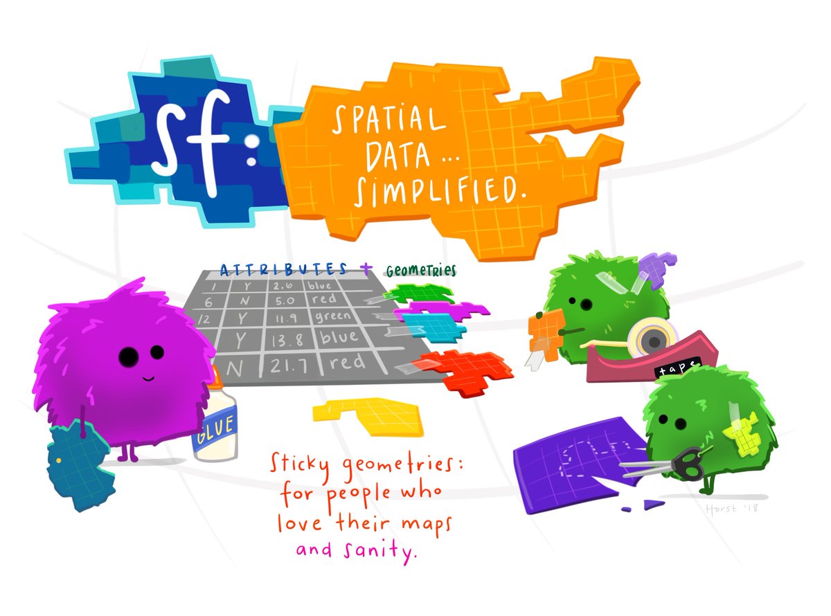
Schematic of the sf data frame, illustration by Allison Horst
SpatialFeatureExperiment (SFE) is a new S4 class built on top of SpatialExperiment
(SPE). SpatialFeatureExperiment incorporates geometries and
geometry operations with the sf package. Examples of
supported geometries are Visium spots represented with polygons
corresponding to their size, cell or nuclei segmentation polygons,
tissue boundary polygons, pathologist annotation of histological
regions, and transcript spots of genes. Using sf,
SpatialFeatureExperiment leverages the GEOS C++ libraries
underlying sf for geometry operations, including algorithms
for for determining whether geometries intersect, finding intersection
geometries, buffering geometries with margins, etc. A schematic of the
SFE object is shown below:
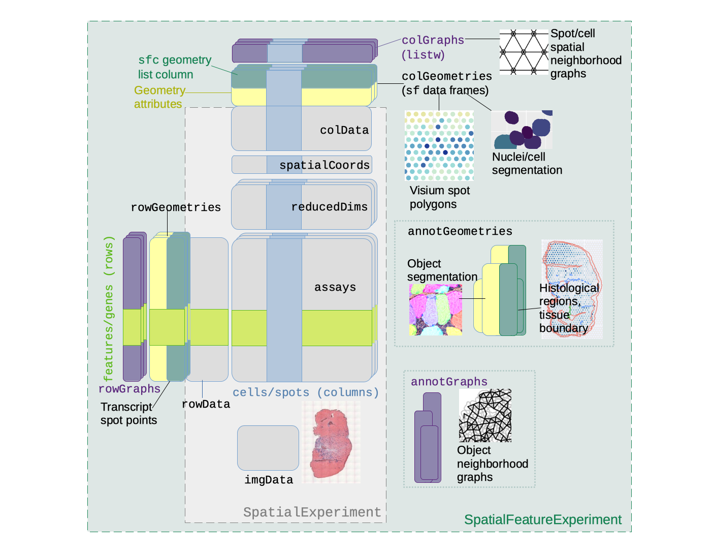
Schematics of the SFE object
Below is a list of SFE features that extend the SPE object:
-
colGeometriesaresfdata frames associated with the entities that correspond to columns of the gene count matrix, such as Visium spots or cells. The geometries in thesfdata frames can be Visium spot centroids, Visium spot polygons, or for datasets with single cell resolution, cell or nuclei segmentations. MultiplecolGeometriescan be stored in the same SFE object, such as one for cell segmentation and another for nuclei segmentation. There can be non-spatial, attribute columns in acolGeometryrather thancolData, because thesfclass allows users to specify how attributes relate to geometries, such as “constant”, “aggregate”, and “identity”. See theagrargument of thest_sfdocumentation. -
colGraphsare spatial neighborhood graphs of cells or spots. The graphs have classlistw(spdeppackage), and thecolPairsofSingleCellExperimentwas not used so no conversion is necessary to use the numerous spatial dependency functions fromspdep, such as those for Moran’s I, Geary’s C, Getis-Ord Gi*, LOSH, etc. Conversion is also not needed for other classical spatial statistics packages such asspatialregandadespatial. -
rowGeometriesare similar tocolGeometries, but support entities that correspond to rows of the gene count matrix, such as genes. A potential use case is to store transcript spots for each gene in smFISH or in situ sequencing based datasets. -
rowGraphsare similar tocolGraphs. A potential use case may be spatial colocalization of transcripts of different genes. -
annotGeometriesaresfdata frames associated with the dataset but not directly with the gene count matrix, such as tissue boundaries, histological regions, cell or nuclei segmentation in Visium datasets, and etc. These geometries are stored in this object to facilitate plotting and usingsffor operations such as to find the number of nuclei in each Visium spot and which histological regions each Visium spot intersects. UnlikecolGeometriesandrowGeometries, the number of rows in thesfdata frames inannotGeometriesis not constrained by the dimension of the gene count matrix and can be arbitrary. -
annotGraphsare similar tocolGraphsandrowGraphs, but are for entities not directly associated with the gene count matrix, such as spatial neighborhood graphs for nuclei in Visium datasets, or other objects like myofibers. These graphs are relevant tospdepanalyses of attributes of these geometries such as spatial autocorrelation in morphological metrics of myofibers and nuclei. With geometry operations withsf, these attributes and results of analyses of these attributes (e.g. spatial regions defined by the attributes) may be related back to gene expression.
library(SpatialFeatureExperiment)
library(SpatialExperiment)
#> Loading required package: SingleCellExperiment
#> Loading required package: SummarizedExperiment
#> Loading required package: MatrixGenerics
#> Loading required package: matrixStats
#>
#> Attaching package: 'MatrixGenerics'
#> The following objects are masked from 'package:matrixStats':
#>
#>     colAlls, colAnyNAs, colAnys, colAvgsPerRowSet, colCollapse,
#>     colCounts, colCummaxs, colCummins, colCumprods, colCumsums,
#>     colDiffs, colIQRDiffs, colIQRs, colLogSumExps, colMadDiffs,
#>     colMads, colMaxs, colMeans2, colMedians, colMins, colOrderStats,
#>     colProds, colQuantiles, colRanges, colRanks, colSdDiffs, colSds,
#>     colSums2, colTabulates, colVarDiffs, colVars, colWeightedMads,
#>     colWeightedMeans, colWeightedMedians, colWeightedSds,
#>     colWeightedVars, rowAlls, rowAnyNAs, rowAnys, rowAvgsPerColSet,
#>     rowCollapse, rowCounts, rowCummaxs, rowCummins, rowCumprods,
#>     rowCumsums, rowDiffs, rowIQRDiffs, rowIQRs, rowLogSumExps,
#>     rowMadDiffs, rowMads, rowMaxs, rowMeans2, rowMedians, rowMins,
#>     rowOrderStats, rowProds, rowQuantiles, rowRanges, rowRanks,
#>     rowSdDiffs, rowSds, rowSums2, rowTabulates, rowVarDiffs, rowVars,
#>     rowWeightedMads, rowWeightedMeans, rowWeightedMedians,
#>     rowWeightedSds, rowWeightedVars
#> Loading required package: GenomicRanges
#> Loading required package: stats4
#> Loading required package: BiocGenerics
#>
#> Attaching package: 'BiocGenerics'
#> The following objects are masked from 'package:stats':
#>
#>     IQR, mad, sd, var, xtabs
#> The following objects are masked from 'package:base':
#>
#>     anyDuplicated, append, as.data.frame, basename, cbind, colnames,
#>     dirname, do.call, duplicated, eval, evalq, Filter, Find, get, grep,
#>     grepl, intersect, is.unsorted, lapply, Map, mapply, match, mget,
#>     order, paste, pmax, pmax.int, pmin, pmin.int, Position, rank,
#>     rbind, Reduce, rownames, sapply, setdiff, sort, table, tapply,
#>     union, unique, unsplit, which.max, which.min
#> Loading required package: S4Vectors
#>
#> Attaching package: 'S4Vectors'
#> The following objects are masked from 'package:base':
#>
#>     expand.grid, I, unname
#> Loading required package: IRanges
#> Loading required package: GenomeInfoDb
#> Loading required package: Biobase
#> Welcome to Bioconductor
#>
#>     Vignettes contain introductory material; view with
#>     'browseVignettes()'. To cite Bioconductor, see
#>     'citation("Biobase")', and for packages 'citation("pkgname")'.
#>
#> Attaching package: 'Biobase'
#> The following object is masked from 'package:MatrixGenerics':
#>
#>     rowMedians
#> The following objects are masked from 'package:matrixStats':
#>
#>     anyMissing, rowMedians
library(SFEData)
library(sf)
#> Linking to GEOS 3.8.0, GDAL 3.0.4, PROJ 6.3.1; sf_use_s2() is TRUE
library(Matrix)
#>
#> Attaching package: 'Matrix'
#> The following object is masked from 'package:S4Vectors':
#>
#>     expand
Object construction
From scratch
An SFE object can be constructed from scratch with the assay
matrices, column metadata, and spatial coordinates. In this toy example,
dgCMatrix is used, but since SFE inherits from
SingleCellExperiment (SCE), other types of arrays supported by SCE such
as delayed arrays should also work.
# Visium barcode location from Space Ranger
data("visium_row_col")
coords1 <- visium_row_col[visium_row_col$col < 6 & visium_row_col$row < 6,]
coords1$row <- coords1$row * sqrt(3)

# Random toy sparse matrix
set.seed(29)
col_inds <- sample(1:13, 13)
row_inds <- sample(1:5, 13, replace = TRUE)
values <- sample(1:5, 13, replace = TRUE)
mat <- sparseMatrix(i = row_inds, j = col_inds, x = values)
colnames(mat) <- coords1$barcode
rownames(mat) <- sample(LETTERS, 5)
That should be sufficient to create an SPE object, and an SFE object,
even though no sf data frame was constructed for the
geometries. The constructor behaves similarly to the SPE constructor.
The centroid coordinates of the Visium spots in the toy example can be
converted into spot polygons with the spotDiameter
argument. Spot diameter in pixels in full resolution image can be found
in the scalefactors_json.json file in Space Ranger
output.
sfe3 <- SpatialFeatureExperiment(list(counts = mat), colData = coords1,
                                spatialCoordsNames = c("col", "row"),
                                spotDiameter = 0.7)
More geometries and spatial graphs can be added after calling the constructor.
Geometries can also be supplied in the constructor.
Space Ranger output
Space Ranger output can be read in a similar manner as in
SpatialExperiment; the returned SFE object has the
spotPoly column geometry for the spot polygons. If the
filtered matrix is read in, then a column graph called
visium will also be present, for the spatial neighborhood
graph of the Visium spots on tissue. The graph is not computed if all
spots are read in regardless of whether they are on tissue.
# Example from SpatialExperiment
dir <- system.file(
  file.path("extdata", "10xVisium"),
  package = "SpatialExperiment")

sample_ids <- c("section1", "section2")
samples <- file.path(dir, sample_ids, "outs")

# The "outs" directory in Space Ranger output
list.files(samples[1])
#> [1] "raw_feature_bc_matrix" "spatial"

# The contents of the "spatial" directory
list.files(file.path(samples[1], "spatial"))
#> [1] "scalefactors_json.json"    "tissue_lowres_image.png"
#> [3] "tissue_positions_list.csv"

# Where the raw gene count matrix is located
file.path(samples[1], "raw_feature_bc_matrix")
#> [1] "/usr/local/lib/R/site-library/SpatialExperiment/extdata/10xVisium/section1/outs/raw_feature_bc_matrix"
(sfe3 <- read10xVisiumSFE(samples, sample_ids, type = "sparse", data = "raw",
                         load = FALSE))
#> class: SpatialFeatureExperiment
#> dim: 50 99
#> metadata(0):
#> assays(1): counts
#> rownames(50): ENSMUSG00000051951 ENSMUSG00000089699 ...
#>   ENSMUSG00000005886 ENSMUSG00000101476
#> rowData names(1): symbol
#> colnames(99): AAACAACGAATAGTTC-1 AAACAAGTATCTCCCA-1 ...
#>   AAAGTCGACCCTCAGT-1-1 AAAGTGCCATCAATTA-1-1
#> colData names(4): in_tissue array_row array_col sample_id
#> reducedDimNames(0):
#> mainExpName: NULL
#> altExpNames(0):
#> spatialCoords names(2) : pxl_row_in_fullres pxl_col_in_fullres
#> imgData names(4): sample_id image_id data scaleFactor
#>
#> Geometries:
#> colGeometries: spotPoly (POLYGON)
#> annotGeometries:  ()
#>
#> Graphs:
#> section1:
#> section2:
Coercion from SpatialExperiment
SPE objects can be coerced into SFE objects. If column geometries or spot diameter are not specified, then a column geometry called “centroids” will be created.
spe <- read10xVisium(samples, sample_ids, type = "sparse", data = "raw",
  images = "lowres", load = FALSE)
For the coercion, column names must not be duplicate.
colnames(spe) <- make.unique(colnames(spe), sep = "-")
rownames(spatialCoords(spe)) <- colnames(spe)
(sfe3 <- toSpatialFeatureExperiment(spe))
#> class: SpatialFeatureExperiment
#> dim: 50 99
#> metadata(0):
#> assays(1): counts
#> rownames(50): ENSMUSG00000051951 ENSMUSG00000089699 ...
#>   ENSMUSG00000005886 ENSMUSG00000101476
#> rowData names(1): symbol
#> colnames(99): AAACAACGAATAGTTC-1 AAACAAGTATCTCCCA-1 ...
#>   AAAGTCGACCCTCAGT-1-1 AAAGTGCCATCAATTA-1-1
#> colData names(4): in_tissue array_row array_col sample_id
#> reducedDimNames(0):
#> mainExpName: NULL
#> altExpNames(0):
#> spatialCoords names(2) : pxl_col_in_fullres pxl_row_in_fullres
#> imgData names(4): sample_id image_id data scaleFactor
#>
#> Geometries:
#> colGeometries: centroids (POINT)
#> annotGeometries:  ()
#>
#> Graphs:
#> section1:
#> section2:
Getters and setters
# Example dataset
(sfe <- McKellarMuscleData(dataset = "small"))
#> snapshotDate(): 2022-07-22
#> see ?SFEData and browseVignettes('SFEData') for documentation
#> loading from cache
#> class: SpatialFeatureExperiment
#> dim: 15123 77
#> metadata(0):
#> assays(1): counts
#> rownames(15123): ENSMUSG00000025902 ENSMUSG00000096126 ...
#>   ENSMUSG00000064368 ENSMUSG00000064370
#> rowData names(6): Ensembl symbol ... vars cv2
#> colnames(77): AAATTACCTATCGATG AACATATCAACTGGTG ... TTCTTTGGTCGCGACG
#>   TTGATGTGTAGTCCCG
#> colData names(12): barcode col ... prop_mito in_tissue
#> reducedDimNames(0):
#> mainExpName: NULL
#> altExpNames(0):
#> spatialCoords names(2) : imageX imageY
#> imgData names(1): sample_id
#>
#> Geometries:
#> colGeometries: spotPoly (POLYGON)
#> annotGeometries: tissueBoundary (POLYGON), myofiber_full (GEOMETRY), myofiber_simplified (GEOMETRY), nuclei (POLYGON), nuclei_centroid (POINT)
#>
#> Graphs:
#> Vis5A:
Geometries
User interfaces to get or set the geometries and spatial graphs
emulate those of reducedDims
in SingleCellExperiment.
Geometries associated with columns of the gene count matrix (cells or
Visium spots) can be get/set with colGeometry. Similarly,
geometries associated with rows of the gene count matrix (genes or
features) can be get/set with rowGeometry, and geometries
associated with the annotations can be get/set with
annotGeometry. Here we demonstrate colGeometry
as the arguments for rowGeometry and
annotGeometry are the same. See the vignette
of SpatialFeatureExperiment for more details.
# Get Visium spot polygons
(spots <- colGeometry(sfe, type = "spotPoly"))
#> Simple feature collection with 77 features and 1 field
#> Geometry type: POLYGON
#> Dimension:     XY
#> Bounding box:  xmin: 5000 ymin: 13000 xmax: 7000 ymax: 15000
#> CRS:           NA
#> First 10 features:
#>                                        geometry sample_id
#> AAATTACCTATCGATG POLYGON ((6472.186 13875.23...     Vis5A
#> AACATATCAACTGGTG POLYGON ((5778.291 13635.43...     Vis5A
#> AAGATTGGCGGAACGT POLYGON ((7000 13809.84, 69...     Vis5A
#> AAGGGACAGATTCTGT POLYGON ((6749.535 13874.64...     Vis5A
#> AATATCGAGGGTTCTC POLYGON ((5500.941 13636.03...     Vis5A
#> AATGATGATACGCTAT POLYGON ((6612.42 14598.82,...     Vis5A
#> AATGATGCGACTCCTG POLYGON ((5501.981 14118.62...     Vis5A
#> AATTCATAAGGGATCT POLYGON ((6889.769 14598.22...     Vis5A
#> ACGAGTACGGATGCCC POLYGON ((5084.397 13395.63...     Vis5A
#> ACGCTAGTGATACACT POLYGON ((5639.096 13394.44...     Vis5A
# Use st_geometry so it won't color by the attributes
plot(st_geometry(spots))
# Setter
colGeometry(sfe, "foobar") <- spots
colGeometryNames gets or sets the names of the
geometries
(cg_names <- colGeometryNames(sfe))
#> [1] "spotPoly" "foobar"
There are shorthands for some specific geometries. For example,
spotPoly(sfe) is equivalent to
colGeometry(sfe, "spotPoly") for Visium spot polygons, and
txSpots(sfe) is equivalent to
rowGeometry(sfe, "txSpots") for transcript spots in single
molecule technologies.
# Getter
(spots <- spotPoly(sfe))
#> Simple feature collection with 77 features and 1 field
#> Geometry type: POLYGON
#> Dimension:     XY
#> Bounding box:  xmin: 5000 ymin: 13000 xmax: 7000 ymax: 15000
#> CRS:           NA
#> First 10 features:
#>                                        geometry sample_id
#> AAATTACCTATCGATG POLYGON ((6472.186 13875.23...     Vis5A
#> AACATATCAACTGGTG POLYGON ((5778.291 13635.43...     Vis5A
#> AAGATTGGCGGAACGT POLYGON ((7000 13809.84, 69...     Vis5A
#> AAGGGACAGATTCTGT POLYGON ((6749.535 13874.64...     Vis5A
#> AATATCGAGGGTTCTC POLYGON ((5500.941 13636.03...     Vis5A
#> AATGATGATACGCTAT POLYGON ((6612.42 14598.82,...     Vis5A
#> AATGATGCGACTCCTG POLYGON ((5501.981 14118.62...     Vis5A
#> AATTCATAAGGGATCT POLYGON ((6889.769 14598.22...     Vis5A
#> ACGAGTACGGATGCCC POLYGON ((5084.397 13395.63...     Vis5A
#> ACGCTAGTGATACACT POLYGON ((5639.096 13394.44...     Vis5A
# Setter
spotPoly(sfe) <- spots
tissueBoundary(sfe) is equivalent to
annotGeometry(sfe, "tissueBoundary").
# Getter
(tb <- tissueBoundary(sfe))
#> Simple feature collection with 1 feature and 2 fields
#> Geometry type: POLYGON
#> Dimension:     XY
#> Bounding box:  xmin: 5094 ymin: 13000 xmax: 7000 ymax: 14969
#> CRS:           NA
#>   ID                       geometry sample_id
#> 7  7 POLYGON ((5094 13000, 5095 ...     Vis5A
plot(st_geometry(tb))
# Setter
tissueBoundary(sfe) <- tb
Spatial graphs
Spatial dependence analyses in the spdep package
requires a spatial neighborhood graph. The
SpatialFeatureExperiment package wraps functions in the
spdep package to find spatial neighborhood graphs. In this
example, triangulation is used to find the spatial graph; many other
methods are also supported, such as k nearest neighbors, distance based
neighbors, and polygon contiguity.
(g <- findSpatialNeighbors(sfe, MARGIN = 2, type = "spotPoly", method = "tri2nb"))
#> Characteristics of weights list object:
#> Neighbour list object:
#> Number of regions: 77
#> Number of nonzero links: 428
#> Percentage nonzero weights: 7.218755
#> Average number of links: 5.558442
#>
#> Weights style: W
#> Weights constants summary:
#>    n   nn S0       S1       S2
#> W 77 5929 77 28.24222 310.1917
This is what the triangulated graph looks like
plot(g, coords = spatialCoords(sfe))
Similar to colGeometry, rowGeometry, and
annotGeometry, the spatial graphs can be get and set with
colGraph, rowGraph, and
annotGraph; the arguments of the graph getters and setters
are the same as those of the geometry getters and setters, so we only
demonstrate colGraph here.
For Visium, spatial neighborhood graph of the hexagonal grid can be found with the known locations of the barcodes.
colGraph(sfe, "visium") <- findVisiumGraph(sfe)This is what the Visium graph looks like
plot(colGraph(sfe, "visium"), coords = spatialCoords(sfe))
Similar to the geometries, the graphs have getters and setters for the names:
colGraphNames(sfe)
#> [1] "visium"
Multiple samples
Thus far, the example dataset used only has one sample. The
SpatialExperiment (SPE) object has a special column in
colData called sample_id, so data from
multiple tissue sections can coexist in the same SPE object for joint
dimension reduction and clustering while keeping the spatial coordinates
separate. It’s important to keep spatial coordinates of different tissue
sections separate because first, the coordinates would only make sense
within the same section, and second, the coordinates from different
sections can have overlapping numeric values.
SFE inherits from SPE, and with geometries and spatial graphs,
sample_id is even more important. The geometry and graph
getter and setter functions shown above have a sample_id
argument, which is optional when only one sample is present in the SFE
object. This argument is mandatory if multiple samples are present, and
can be a character vector for multiple samples or “all” for all samples.
Below are examples of using the getters and setters for multiple
samples.
# Construct toy dataset with 2 samples
sfe1 <- McKellarMuscleData(dataset = "small")
#> snapshotDate(): 2022-07-22
#> see ?SFEData and browseVignettes('SFEData') for documentation
#> loading from cache
sfe2 <- McKellarMuscleData(dataset = "small2")
#> snapshotDate(): 2022-07-22
#> see ?SFEData and browseVignettes('SFEData') for documentation
#> loading from cache
spotPoly(sfe2)$sample_id <- "sample02"
(sfe_combined <- cbind(sfe1, sfe2))
#> class: SpatialFeatureExperiment
#> dim: 15123 149
#> metadata(0):
#> assays(1): counts
#> rownames(15123): ENSMUSG00000025902 ENSMUSG00000096126 ...
#>   ENSMUSG00000064368 ENSMUSG00000064370
#> rowData names(6): Ensembl symbol ... vars cv2
#> colnames(149): AAATTACCTATCGATG AACATATCAACTGGTG ... TTCCTCGGACTAACCA
#>   TTCTGACCGGGCTCAA
#> colData names(12): barcode col ... prop_mito in_tissue
#> reducedDimNames(0):
#> mainExpName: NULL
#> altExpNames(0):
#> spatialCoords names(2) : imageX imageY
#> imgData names(1): sample_id
#>
#> Geometries:
#> colGeometries: spotPoly (POLYGON)
#> annotGeometries: tissueBoundary (GEOMETRY), myofiber_full (GEOMETRY), myofiber_simplified (GEOMETRY), nuclei (POLYGON), nuclei_centroid (POINT)
#>
#> Graphs:
#> Vis5A:
#> sample02:
Use the sampleIDs function to see the names of all
samples
sampleIDs(sfe_combined)
#> [1] "Vis5A"    "sample02"
# Only get the geometries for the second sample
(spots2 <- colGeometry(sfe_combined, "spotPoly", sample_id = "sample02"))
#> Simple feature collection with 72 features and 1 field
#> Geometry type: POLYGON
#> Dimension:     XY
#> Bounding box:  xmin: 6000 ymin: 7025.865 xmax: 8000 ymax: 9000
#> CRS:           NA
#> First 10 features:
#>                  sample_id                       geometry
#> AACACACGCTCGCCGC  sample02 POLYGON ((6597.869 7842.575...
#> AACCGCTAAGGGATGC  sample02 POLYGON ((6724.811 9000, 67...
#> AACGCTGTTGCTGAAA  sample02 POLYGON ((6457.635 7118.991...
#> AACGGACGTACGTATA  sample02 POLYGON ((6737.064 8083.571...
#> AATAGAATCTGTTTCA  sample02 POLYGON ((7570.153 8564.368...
#> ACAAATCGCACCGAAT  sample02 POLYGON ((8000 7997.001, 79...
#> ACAATTGTGTCTCTTT  sample02 POLYGON ((6043.169 7843.77,...
#> ACAGGCTTGCCCGACT  sample02 POLYGON ((7428.88 7358.195,...
#> ACCAGTGCGGGAGACG  sample02 POLYGON ((6460.753 8566.757...
#> ACCCTCCCTTGCTATT  sample02 POLYGON ((7847.503 8563.771...
Sample IDs can also be changed, with the changeSampleIDs
function, with a named vector whose names are the old names and values
are the new names.
sfe_combined <- changeSampleIDs(sfe_combined, replacement = c(Vis5A = "foo", sample02 = "bar"))
sampleIDs(sfe_combined)
#> [1] "foo" "bar"
Operations
Non-geometric
SFE objects can be concatenated with cbind, as was done
just now to create a toy example with 2 samples.
sfe_combined <- cbind(sfe1, sfe2)The SFE object can also be subsetted like a matrix, like an SCE
object. More complexity arises when it comes to the spatial graphs. The
drop argument of the SFE method [ determines
what to do with the spatial graphs. If drop = TRUE, then
all spatial graphs will be removed, since the graphs with nodes and
edges that have been removed are no longer valid. If
drop = FALSE, which is the default, then the spatial graphs
will be reconstructed with the remaining nodes after subsetting.
Reconstruction would only work when the original graphs were constructed
with findSpatialNeighbors or findVisiumGraph
in this package, which records the method and parameters used to
construct the graphs. If reconstruction fails, then a warning will be
issued and the graphs removed.
(sfe_subset <- sfe[1:10, 1:10, drop = TRUE])
#> Node indices in the graphs are no longer valid after subsetting. Dropping all row and col graphs.
#> class: SpatialFeatureExperiment
#> dim: 10 10
#> metadata(0):
#> assays(1): counts
#> rownames(10): ENSMUSG00000025902 ENSMUSG00000096126 ...
#>   ENSMUSG00000090031 ENSMUSG00000033740
#> rowData names(6): Ensembl symbol ... vars cv2
#> colnames(10): AAATTACCTATCGATG AACATATCAACTGGTG ... ACGAGTACGGATGCCC
#>   ACGCTAGTGATACACT
#> colData names(12): barcode col ... prop_mito in_tissue
#> reducedDimNames(0):
#> mainExpName: NULL
#> altExpNames(0):
#> spatialCoords names(2) : imageX imageY
#> imgData names(1): sample_id
#>
#> Geometries:
#> colGeometries: spotPoly (POLYGON), foobar (POLYGON)
#> annotGeometries: tissueBoundary (POLYGON), myofiber_full (GEOMETRY), myofiber_simplified (GEOMETRY), nuclei (POLYGON), nuclei_centroid (POINT)
#>
#> Graphs:
#> Vis5A:
# Will give warning because graph reconstruction fails
sfe_subset <- sfe[1:10, 1:10]
Geometric
Just like sf data frames, SFE objects can be subsetted
by a geometry and a predicate relating geometries. For example, if all
Visium spots were read into an SFE object regardless of whether they are
in tissue, and the tissueBoundary annotation geometry is
provided, then the tissue boundary geometry can be used to subset the
SFE object to obtain a new SFE object with only spots on tissue. Loupe
does not give the tissue boundary polygon; such polygon can be obtained
by thresholding the H&E image and converting the mask into polygons
with OpenCV or the terra R package, or by manual annotation
in QuPath or LabKit (the latter needs to be converted into polygon).
Use the crop function to directly get the subsetted SFE
object. Note that in this version of this package, crop
does NOT crop the image.
# Before
plot(st_geometry(tissueBoundary(sfe)))
plot(spotPoly(sfe), col = "gray", add = TRUE)
sfe_in_tissue <- crop(sfe, y = tissueBoundary(sfe), colGeometryName = "spotPoly")Note that for large datasets with many geometries, cropping can take a while to run.
# After
plot(st_geometry(tissueBoundary(sfe)))
plot(spotPoly(sfe_in_tissue), col = "gray", add = TRUE)
crop can also be used in the conventional sense of
cropping, i.e. specifying a bounding box.
sfe_cropped <- crop(sfe, colGeometryName = "spotPoly", sample_id = "Vis5A",
                    xmin = 5500, xmax = 6500, ymin = 13500, ymax = 14500)
The colGeometryName is used to determine which columns
in the gene count matrix to keep. All geometries in the SFE object will
be subsetted so only portions intersecting y or the
bounding box are kept. Since the intersection operation can produce a
mixture of geometry types, such as intersection of two polygons
producing polygons, points, and lines, the geometry types of the
sf data frames after subsetting may be different from those
of the originals.
The cropping is done independently for each sample_id,
and only on sample_ids specified. Again,
sample_id is optional when there is only one sample in the
SFE object.
Geometry predicates and operations can also be performed to return
the results without subsetting an SFE object. For example, one may want
a logical vector indicating whether each Visium spot intersects the
tissue, or a numeric vector of how many nuclei there are in each Visium
spot. Or get the intersections between each Visium spot and nuclei.
Again, the geometry predicates and operations are performed
independently for each sample, and the sample_id argument
is optional when there is only one sample.
# Get logical vector of whether each Visium spot intersects tissue
colData(sfe)$in_tissue <- annotPred(sfe, colGeometryName = "spotPoly",
                                    annotGeometryName = "tissueBoundary",
                                    sample_id = "Vis5A")
# Get the number of nuclei per Visium spot
colData(sfe)$n_nuclei <- annotNPred(sfe, "spotPoly", annotGeometryName = "nuclei")
# Get geometries of intersections of Visium spots and myofibers
spot_intersections <- annotOp(sfe, colGeometryName = "spotPoly",
                              annotGeometryName = "myofiber_simplified")
Sometimes the spatial coordinates of different samples can take very
different values. The values can be made more comparable by moving all
tissues so the bottom left corner of the bounding box would be at the
origin, which would facilitate plotting and comparison across samples
with geom_sf and facet_*.
To find the bounding box of all geometries in each sample of an SFE object:
bbox(sfe, sample_id = "Vis5A")
#>  xmin  ymin  xmax  ymax
#>  5000 13000  7000 15000
To move the coordinates:
sfe_moved <- removeEmptySpace(sfe, sample_id = "Vis5A")
bbox(sfe_moved, sample_id = "Vis5A")
#> xmin ymin xmax ymax
#>    0    0 2000 2000
The original bounding box before moving is stored within the SFE
object, which can be read by dimGeometry setters so newly
added geometries can have coordinates moved as well; this behavior can
be turned off with the optional argument translate = FALSE
in dimGeometry setters.
Limitations
- Only 2D data is supported for now.
- Geometric operation do not change the SPE
ImgData. - Does not support raster data or
spatstatspatial point process analyses.
Session info
sessionInfo()
#> R version 4.2.0 (2022-04-22)
#> Platform: x86_64-pc-linux-gnu (64-bit)
#> Running under: Ubuntu 20.04.4 LTS
#>
#> Matrix products: default
#> BLAS:   /usr/lib/x86_64-linux-gnu/openblas-pthread/libblas.so.3
#> LAPACK: /usr/lib/x86_64-linux-gnu/openblas-pthread/liblapack.so.3
#>
#> locale:
#>  [1] LC_CTYPE=en_US.UTF-8       LC_NUMERIC=C
#>  [3] LC_TIME=en_US.UTF-8        LC_COLLATE=en_US.UTF-8
#>  [5] LC_MONETARY=en_US.UTF-8    LC_MESSAGES=en_US.UTF-8
#>  [7] LC_PAPER=en_US.UTF-8       LC_NAME=C
#>  [9] LC_ADDRESS=C               LC_TELEPHONE=C
#> [11] LC_MEASUREMENT=en_US.UTF-8 LC_IDENTIFICATION=C
#>
#> attached base packages:
#> [1] stats4    stats     graphics  grDevices utils     datasets  methods
#> [8] base
#>
#> other attached packages:
#>  [1] Matrix_1.4-1                    sf_1.0-8
#>  [3] SFEData_0.99.0                  SpatialExperiment_1.7.0
#>  [5] SingleCellExperiment_1.19.0     SummarizedExperiment_1.27.1
#>  [7] Biobase_2.57.1                  GenomicRanges_1.49.0
#>  [9] GenomeInfoDb_1.33.3             IRanges_2.31.0
#> [11] S4Vectors_0.35.1                BiocGenerics_0.43.0
#> [13] MatrixGenerics_1.9.1            matrixStats_0.62.0
#> [15] SpatialFeatureExperiment_0.99.0
#>
#> loaded via a namespace (and not attached):
#>   [1] rjson_0.2.21                  deldir_1.0-6
#>   [3] ellipsis_0.3.2                class_7.3-20
#>   [5] rprojroot_2.0.3               scuttle_1.7.2
#>   [7] XVector_0.37.0                fs_1.5.2
#>   [9] proxy_0.4-27                  bit64_4.0.5
#>  [11] AnnotationDbi_1.59.1          interactiveDisplayBase_1.35.0
#>  [13] fansi_1.0.3                   codetools_0.2-18
#>  [15] R.methodsS3_1.8.2             sparseMatrixStats_1.9.0
#>  [17] cachem_1.0.6                  knitr_1.39
#>  [19] jsonlite_1.8.0                dbplyr_2.2.1
#>  [21] png_0.1-7                     R.oo_1.25.0
#>  [23] shiny_1.7.2                   HDF5Array_1.25.1
#>  [25] BiocManager_1.30.18           compiler_4.2.0
#>  [27] httr_1.4.3                    dqrng_0.3.0
#>  [29] assertthat_0.2.1              fastmap_1.1.0
#>  [31] limma_3.53.5                  cli_3.3.0
#>  [33] later_1.3.0                   s2_1.1.0
#>  [35] htmltools_0.5.3               tools_4.2.0
#>  [37] glue_1.6.2                    GenomeInfoDbData_1.2.8
#>  [39] dplyr_1.0.9                   rappdirs_0.3.3
#>  [41] wk_0.6.0                      Rcpp_1.0.9
#>  [43] jquerylib_0.1.4               pkgdown_2.0.6
#>  [45] raster_3.5-21                 Biostrings_2.65.1
#>  [47] vctrs_0.4.1                   rhdf5filters_1.9.0
#>  [49] spdep_1.2-4                   ExperimentHub_2.5.0
#>  [51] DelayedMatrixStats_1.19.0     xfun_0.31
#>  [53] stringr_1.4.0                 beachmat_2.13.4
#>  [55] mime_0.12                     lifecycle_1.0.1
#>  [57] terra_1.5-34                  AnnotationHub_3.5.0
#>  [59] edgeR_3.39.3                  zlibbioc_1.43.0
#>  [61] promises_1.2.0.1              ragg_1.2.2
#>  [63] parallel_4.2.0                rhdf5_2.41.1
#>  [65] yaml_2.3.5                    curl_4.3.2
#>  [67] memoise_2.0.1                 sass_0.4.2
#>  [69] stringi_1.7.8                 RSQLite_2.2.15
#>  [71] BiocVersion_3.16.0            highr_0.9
#>  [73] desc_1.4.1                    e1071_1.7-11
#>  [75] filelock_1.0.2                boot_1.3-28
#>  [77] BiocParallel_1.31.10          spData_2.0.1
#>  [79] rlang_1.0.4                   pkgconfig_2.0.3
#>  [81] systemfonts_1.0.4             bitops_1.0-7
#>  [83] evaluate_0.15                 lattice_0.20-45
#>  [85] purrr_0.3.4                   Rhdf5lib_1.19.2
#>  [87] bit_4.0.4                     tidyselect_1.1.2
#>  [89] magrittr_2.0.3                R6_2.5.1
#>  [91] magick_2.7.3                  generics_0.1.3
#>  [93] DelayedArray_0.23.0           DBI_1.1.3
#>  [95] pillar_1.8.0                  units_0.8-0
#>  [97] KEGGREST_1.37.3               RCurl_1.98-1.7
#>  [99] sp_1.5-0                      tibble_3.1.8
#> [101] crayon_1.5.1                  DropletUtils_1.17.0
#> [103] KernSmooth_2.23-20            utf8_1.2.2
#> [105] BiocFileCache_2.5.0           rmarkdown_2.14
#> [107] locfit_1.5-9.6                grid_4.2.0
#> [109] blob_1.2.3                    digest_0.6.29
#> [111] classInt_0.4-7                xtable_1.8-4
#> [113] httpuv_1.6.5                  R.utils_2.12.0
#> [115] textshaping_0.3.6             bslib_0.4.0