Introduction
In single cell RNA-seq (scRNA-seq), data and metadata can be
represented with SingleCellExperiment or
Seurat objects, and basic exploratory data analyses and
visualization performed with scater, scran,
and scuttle, or Seurat. The
SpatialFeatureExperiment package and S4 class extending
SpatialExperiment and SingleCellExperiment
brings EDA methods for vector spatial data to spatial transcriptomics.
Voyager to SpatialFeatureExperiment is just
like scater, scran, and scuttle
to SingleCellExperiment, implementing basic exploratory
spatial data analysis (ESDA) and visualization methods.
Tobler’s first law of geography:
Everything is related to everything else. But near things are more related than distant things.
Non-spatial statistical methods often assume that the samples (cells, spots) are independent, which is not the case in spatial data, where nearby samples tend to be more similar (i.e. positive spatial autocorrelation; negative spatial autocorrelation is when nearby samples tend to be more dissimilar, like a checkered pattern). Much of ESDA is dedicated to spatial autocorrelation, such as finding whether it is present, and if so what’s its length scale.
This part of the workshop gives an overview of some ESDA methods,
functionalities of the Voyager package, and applications of
the SpatialFeatureExperiment class with a published Visium
dataset.
library(Voyager)
library(SpatialFeatureExperiment)
library(scater)
#> Loading required package: SingleCellExperiment
#> Loading required package: SummarizedExperiment
#> Loading required package: MatrixGenerics
#> Loading required package: matrixStats
#>
#> Attaching package: 'MatrixGenerics'
#> The following objects are masked from 'package:matrixStats':
#>
#>     colAlls, colAnyNAs, colAnys, colAvgsPerRowSet, colCollapse,
#>     colCounts, colCummaxs, colCummins, colCumprods, colCumsums,
#>     colDiffs, colIQRDiffs, colIQRs, colLogSumExps, colMadDiffs,
#>     colMads, colMaxs, colMeans2, colMedians, colMins, colOrderStats,
#>     colProds, colQuantiles, colRanges, colRanks, colSdDiffs, colSds,
#>     colSums2, colTabulates, colVarDiffs, colVars, colWeightedMads,
#>     colWeightedMeans, colWeightedMedians, colWeightedSds,
#>     colWeightedVars, rowAlls, rowAnyNAs, rowAnys, rowAvgsPerColSet,
#>     rowCollapse, rowCounts, rowCummaxs, rowCummins, rowCumprods,
#>     rowCumsums, rowDiffs, rowIQRDiffs, rowIQRs, rowLogSumExps,
#>     rowMadDiffs, rowMads, rowMaxs, rowMeans2, rowMedians, rowMins,
#>     rowOrderStats, rowProds, rowQuantiles, rowRanges, rowRanks,
#>     rowSdDiffs, rowSds, rowSums2, rowTabulates, rowVarDiffs, rowVars,
#>     rowWeightedMads, rowWeightedMeans, rowWeightedMedians,
#>     rowWeightedSds, rowWeightedVars
#> Loading required package: GenomicRanges
#> Loading required package: stats4
#> Loading required package: BiocGenerics
#>
#> Attaching package: 'BiocGenerics'
#> The following objects are masked from 'package:stats':
#>
#>     IQR, mad, sd, var, xtabs
#> The following objects are masked from 'package:base':
#>
#>     anyDuplicated, append, as.data.frame, basename, cbind, colnames,
#>     dirname, do.call, duplicated, eval, evalq, Filter, Find, get, grep,
#>     grepl, intersect, is.unsorted, lapply, Map, mapply, match, mget,
#>     order, paste, pmax, pmax.int, pmin, pmin.int, Position, rank,
#>     rbind, Reduce, rownames, sapply, setdiff, sort, table, tapply,
#>     union, unique, unsplit, which.max, which.min
#> Loading required package: S4Vectors
#>
#> Attaching package: 'S4Vectors'
#> The following objects are masked from 'package:base':
#>
#>     expand.grid, I, unname
#> Loading required package: IRanges
#> Loading required package: GenomeInfoDb
#> Loading required package: Biobase
#> Welcome to Bioconductor
#>
#>     Vignettes contain introductory material; view with
#>     'browseVignettes()'. To cite Bioconductor, see
#>     'citation("Biobase")', and for packages 'citation("pkgname")'.
#>
#> Attaching package: 'Biobase'
#> The following object is masked from 'package:MatrixGenerics':
#>
#>     rowMedians
#> The following objects are masked from 'package:matrixStats':
#>
#>     anyMissing, rowMedians
#> Loading required package: scuttle
#> Loading required package: ggplot2
library(scran)
library(SFEData)
library(sf)
#> Linking to GEOS 3.8.0, GDAL 3.0.4, PROJ 6.3.1; sf_use_s2() is TRUE
library(ggplot2)
library(scales)
library(patchwork)
library(BiocParallel)
library(bluster)
theme_set(theme_bw(10))
Dataset
The dataset used in this vignette comes from Large-scale
integration of single-cell transcriptomic data captures transitional
progenitor states in mouse skeletal muscle regeneration. Notexin was
injected into the tibialis anterior muscle to induce injury, and the
healing muscle was collected 2, 5, and 7 days post injury for Visium.
The dataset here is from the 2 day timepoint. The dataset is in a
SpatialFeatureExperiment (SFE) object.
The gene count matrix was directly downloaded from GEO. All 4992 spots, whether in tissue or not, are included. The H&E image was used for nuclei and myofiber segmentation. A subset of nuclei from randomly selected regions from all 3 timepoints were manually annotated to train a StarDist model to segment the rest of the nuclei, and the myofibers were all manually segmented.
Tissue boundary, nuclei, myofiber, and Visium spot polygons are
stored as sf data frames in the SFE object. See the
vignette of the SpatialFeatureExperiment for more details
on the structure of the SFE object. The SFE object of this dataset is
provided in the SFEData package.
(sfe <- McKellarMuscleData("full"))
#> snapshotDate(): 2022-07-22
#> see ?SFEData and browseVignettes('SFEData') for documentation
#> loading from cache
#> class: SpatialFeatureExperiment
#> dim: 15123 4992
#> metadata(0):
#> assays(1): counts
#> rownames(15123): ENSMUSG00000025902 ENSMUSG00000096126 ...
#>   ENSMUSG00000064368 ENSMUSG00000064370
#> rowData names(6): Ensembl symbol ... vars cv2
#> colnames(4992): AAACAACGAATAGTTC AAACAAGTATCTCCCA ... TTGTTTGTATTACACG
#>   TTGTTTGTGTAAATTC
#> colData names(12): barcode col ... prop_mito in_tissue
#> reducedDimNames(0):
#> mainExpName: NULL
#> altExpNames(0):
#> spatialCoords names(2) : imageX imageY
#> imgData names(1): sample_id
#>
#> Geometries:
#> colGeometries: spotPoly (POLYGON)
#> annotGeometries: tissueBoundary (POLYGON), myofiber_full (POLYGON), myofiber_simplified (POLYGON), nuclei (POLYGON), nuclei_centroid (POINT)
#>
#> Graphs:
#> Vis5A: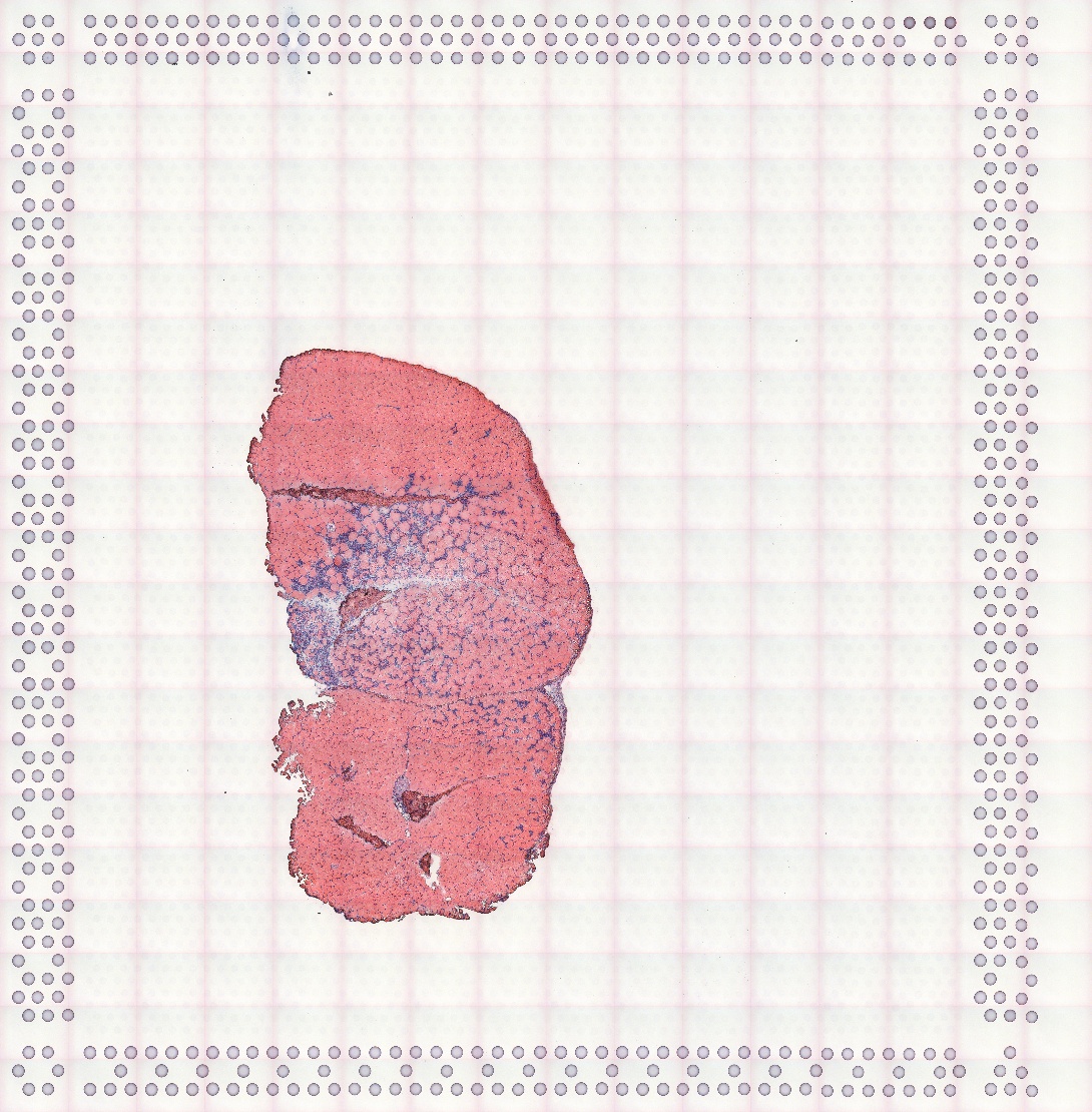
Low resolution H&E image of the tissue section
Exploratory data analysis
Spots in tissue
While the example dataset has all Visium spots whether on tissue or not, only spots that intersect tissue will be used for further analyses.
names(colData(sfe))
#>  [1] "barcode"   "col"       "row"       "x"         "y"         "dia"
#>  [7] "tissue"    "sample_id" "nCounts"   "nGenes"    "prop_mito" "in_tissue"
Total UMI counts (nCounts), number of genes detected per
spot (nGenes), and proportion of mitochondrially encoded
counts (prop_mito) have been precomputed and are in
colData(sfe). The plotSpatialFeature function
plots any gene, colData values, and geometry attributes in
colGeometry and annotGeometry in space. The
Visium spots are plotted as polygons reflecting their actual size
relative to the tissue, rather than points as in other packages that
plot Visium data. Behind the scene, geom_sf is used to plot
the geometries.
The tissue boundary was found by thresholding the H&E image and
removing small polygons that are most likely debris. The
in_tissue column of colData(sfe) indicates
which Visium spot polygon intersects the tissue polygon; this can be
found with SpatialFeatureExperiment::annotPred().
While scran is used for data normalization here for
demonstration purposes and to make the data more normally distributed,
we do not mean that it is the best practice in normalizing spatial
transcriptomics data, as we don’t know what the best practice really
should be. As seen in the nCounts plot in space above,
spatial autocorrelation is evident. In Visium, reverse transcription
occurs in situ on the spots, but PCR amplification occurs after the cDNA
is dissociated from the spots. Then artifacts introduced from the
amplification step would not be spatial. Spatial artifacts may arise
from diffusion of transcripts to adjacent spots and tissue
permeablization. However, given how the total counts seem to correspond
to histological regions, the total counts may have a biological
component and hence should not be treated as a technical artifact to be
normalized away as in scRNA-seq data normalization methods.
sfe_tissue <- sfe[,colData(sfe)$in_tissue]
sfe_tissue <- sfe_tissue[rowSums(counts(sfe_tissue)) > 0,]
clusters <- quickCluster(sfe_tissue)
sfe_tissue <- computeSumFactors(sfe_tissue, clusters=clusters)
#> Warning in (function (x, sizes, min.mean = NULL, positive = FALSE, scaling =
#> NULL) : encountered non-positive size factor estimates
sfe_tissue <- logNormCounts(sfe_tissue)
Myofiber and nuclei segmentation polygons are available in this
dataset, in the field annotGeometries. Myofibers were
manually segmented, and nuclei were segmented with StarDist,
trained with a manually segmented subset.
annotGeometryNames(sfe_tissue)
#> [1] "tissueBoundary"      "myofiber_full"       "myofiber_simplified"
#> [4] "nuclei"              "nuclei_centroid"
From myofibers and nuclei to Visium spots
The plotSpatialFeature function can also be used to plot
attributes of geometries, i.e. the non-geometry columns in the
sf data frames in the rowGeometries,
colGeometries, or annotGeometries fields in
the SFE object. For rowGeometries and
colGeometries, such columns associated with the
sf data frames rather than rowData or
colData are allowed because one can specify how these
columns associate with the geometries (see st_agr
and documentation
of st_sf). When an attribute of an
annotGeometry is plotted along side gene expression or
colData or colGeometry attribute, the
annotGeometry attribute is plotted with a different color
palette to distinguish from the column associated values.
Here, from the annotGeometries, the myofiber polygons
are plotted, colored by cross section area as observed in this tissue
section. The aes_use argument is set to color
rather than fill (default for polygons) to only plot the
Visium spot outlines to make the myofiber polygons more visible. The
fill argument is set to NA to make the Visium
spots look hollow, and the size argument controls the
thickness of the outlines. The annot_aes argument specifies
which column in the annotGeometry to use to specify the
values of an aesthstic, just like aes in
ggplot2 (aes_string to be precise, since
tidyeval is not used here). The annot_fixed
argument (not used here) can set the fixed size, alpha, color, and etc.
for the annotGeometry.
plotSpatialFeature(sfe_tissue, features = "nCounts",
                   colGeometryName = "spotPoly",
                   annotGeometryName = "myofiber_simplified",
                   annot_aes = list(fill = "area"),
                   aes_use = "color", size = 0.5, fill = NA)
The larger myofibers seem to have fewer total counts, possibly because the larger size of these myofibers dilute the transcripts. If this is the case, then data normalization would be relevant to correct for this.
With SpatialFeatureExperiment, we can find the number of
myofibers and nuclei that intersect each Visium spot. The predicate can
be anything
implemented in sf, so for example, the number of nuclei
fully covered by each Visium spot can also be found. The default
predicate is st_intersects.
colData(sfe_tissue)$n_myofibers <-
  annotNPred(sfe_tissue, colGeometryName = "spotPoly",
             annotGeometryName = "myofiber_simplified")
plotSpatialFeature(sfe_tissue, features = "n_myofibers",
                   colGeometryName = "spotPoly")
There is no one to one mapping between Visium spots and myofibers.
However, we may want to relate attributes of myofibers to gene
expression detected at the Visium spots. One way to do so is to
summarize the attributes of all myofibers that intersect (or choose
another better predicate implemented in sf) each spot, such
as to calculate the mean, median, or sum. This can be done with the
annotSummary function in
SpatialFeatureExperiment. The default predicate is
st_intersects, and the default summary function is
mean.
colData(sfe_tissue)$mean_myofiber_area <-
  annotSummary(sfe_tissue, "spotPoly", "myofiber_simplified",
               annotColNames = "area")[,1] # it always returns a data frame
# The gray spots don't intersect any myofiber
plotSpatialFeature(sfe_tissue, "mean_myofiber_area", "spotPoly")
Now we can see how the mean area of myofibers intersecting each Visium spot relates to other aspects of the spots such as total counts and gene expression.
The NAs are for spots not intersecting any myofibers, e.g. those in the inflammatory region.
Myofiber types
Marker genes: Myh7 (Type I, slow twitch, aerobic), Myh2 (Type IIa, fast twitch, somewhat aerobic), Myh4 (Type IIb, fast twitch, anareobic), Myh1 (Type IIx, fast twitch, anaerobic), from this protocol
markers <- c(I = "Myh7", IIa = "Myh2", IIb = "Myh4", IIx = "Myh1")First look at Type I myofibers. This is a fast twitch muscle, so we
don’t expect many slow twitch Type I myofibers. Row names in
sfe_tissue are Ensembl IDs, to avoid ambiguity as sometimes
multiple Ensembl IDs have the same gene symbol and some genes have
aliases in symbol. However, gene symbols are shorter and more human
readable than Ensembl IDs, and are nice to show on plots. In the
plotSpatialFeature function and other functions in
Voyager, even when the actual row names are Ensembl IDs,
the features argument can take gene symbols if there is a
column called “symbols” in rowData(sfe), where the function
converts the gene symbols to Ensembl IDs. By default, gene symbols are
shown on the plot, but the show_symbol argument can be set
to FALSE to show Ensembl IDs instead. If one gene symbol
matches multiple Ensembl IDs in the dataset, then a warning will be
given.
The exprs_values argument specifies the assay to use,
which is by default “logcounts”, i.e. the log normalized data. This
default may or may not be best practice given that total UMI counts may
have biological relevance in spatial data. Therefore we are plotting
both the raw counts and the log normalized counts here.
# Function specific for this vignette, with some hard coded values
plot_counts_logcounts <- function(sfe, feature) {
  p1 <- plotSpatialFeature(sfe, feature, "spotPoly",
                   annotGeometryName = "myofiber_simplified",
                   annot_aes = list(fill = "area"), aes_use = "color",
                   fill = NA, size = 0.5, show_symbol = TRUE,
                   exprs_values = "counts") +
    ggtitle("Raw counts")
  p2 <- plotSpatialFeature(sfe, feature, "spotPoly",
                   annotGeometryName = "myofiber_simplified",
                   annot_aes = list(fill = "area"), aes_use = "color",
                   fill = NA, size = 0.5, show_symbol = TRUE,
                   exprs_values = "logcounts") +
    ggtitle("Log normalized counts")
  p1 + p2 +
    plot_annotation(title = feature)
}
plot_counts_logcounts(sfe_tissue, markers["I"])
Marker gene for type IIa myofibers is shown here. Those interested may change the code to plot markers for tyle IIb and IIx myofibers.
plot_counts_logcounts(sfe_tissue, markers["IIa"])
Type IIa myofibers also tend to be clustered together on left side of the tissue.
As SFE inherits from SCE, the non-spatial EDA plots from the
scater package can still be used.
gene_id <- rownames(sfe_tissue)[rowData(sfe_tissue)$symbol == markers["IIa"]]
plotColData(sfe_tissue, x = "mean_myofiber_area", y = "prop_mito",
            colour_by = gene_id, by_exprs_values = "logcounts")
#> Warning: Removed 36 rows containing missing values (geom_point).
Plotting proportion of mitochondrial counts vs. mean myofiber area, we see two clusters, one with higher proportion of mitochondrial counts and smaller area, and another with lower proportion of mitochondrial counts and on average slightly larger area. Type IIa myofibers tend to have smaller area and larger proportion of mitochondrial counts.
Spatial neighborhood graphs
A spatial neighborhood graph is required to compute spatial
dependency metrics such as Moran’s I and Geary’s C. The
SpatialFeatureExperiment package wraps methods in
spdep to find spatial neighborhood graphs, which are stored
within the SFE object (see spdep documentation for gabrielneigh,
knearneigh,
poly2nb,
and tri2nb).
The Voyager package then uses these graphs for spatial
dependency analyses, again based on spdep in this first
version, but methods from other geospatial packages, some of which also
use the spatial neighborhood graphs, may be added later as needed.
For Visium, where the spots are in a hexagonal grid, the spatial
neighborhood graph is straightforward. However, for spatial technologies
with single cell resolution (e.g. MERFISH) and in this dataset, the
myofibers and nuclei, many different methods can be used to find the
spatial neighborhood graph. Here for myofibers, the method “poly2nb”
identifies myofiber polygons that physically touch each other.
zero.policy = TRUE will allow singletons, i.e. nodes
without neighbors in the graph; in the inflamed region, there are more
singletons. We have not yet benchmarked which spatial neighborhood
method is the “best” in which situation; the particular method used here
is for demonstration purpose and may or may not be best practice.
colGraph(sfe_tissue, "visium") <- findVisiumGraph(sfe_tissue)
annotGraph(sfe_tissue, "myofiber_poly2nb") <-
  findSpatialNeighbors(sfe_tissue, type = "myofiber_simplified", MARGIN = 3,
                       method = "poly2nb", zero.policy = TRUE)
The plotColGraph function plots the graph in space
associated with a colGeometry, along with the geometry of
interest.
plotColGraph(sfe_tissue, colGraphName = "visium", colGeometryName = "spotPoly")
Similarly, the plotAnnotGraph function plots the graph
associated with an annotGeometry, along with the geometry
of interest.
plotAnnotGraph(sfe_tissue, annotGraphName = "myofiber_poly2nb",
               annotGeometryName = "myofiber_simplified")
There is no plotRowGraph yet since we haven’t worked
with a dataset where spatial graphs related to genes are relevant,
although the SFE object supports row graphs.
Exploratory spatial data analysis
All spatial autocorrelation metrics in this package can be computed
directly on a vector or a matrix rather than an SFE object. The user
interface emulates those of dimension reductions in the
scater package (e.g. calculateUMAP that takes
in a matrix or SCE object and returns a matrix, and runUMAP
that takes in an SCE object and adds the results to the
reducedDims field of the SCE object). So
calculate* functions take in a matrix or an SFE object and
directly return the results (format of the results depends on the
structure of the results), while run* functions take in an
SFE object and add the results to the object. In addition,
colData* functions compute the metrics for numeric
variables in colData. colGeometry* functions
compute the metrics for numeric columns in a colGeometry.
annotGeometry* functions compute the metrics for numeric
columns in a annotGeometry.
Univariate
In this first version, Voyager only supports univariate
global spatial autocorrelation implemented in spdep for
ESDA: Moran’s I and Geary’s C, permutation testing for Moran’s I and
Geary’s C, Moran plot, and correlograms. In addition, beyond
spdep, Voyager can cluster Moran plots and
correlograms. Plotting functions taking in SFE objects are implemented
to plot the results with ggplot2 and with more
customization options than spdep plotting functions.
To demonstrate spatial autocorrelation in gene expression, top highly
variable genes (HVGs) are used. The HVGs are found with the
scran method.
dec <- modelGeneVar(sfe_tissue)
hvgs <- getTopHVGs(dec, n = 50)
Moran’s I
There are several ways to quantify spatial autocorrelation, the most common of which is Moran’s I:
\[ I = \frac{n}{\sum_{i=1}^n \sum_{j=1}^n w_{ij}} \frac{\sum_{i=1}^n \sum_{j=1}^n w_{ij} (x_i - \bar{x})(x_j - \bar{x})}{\sum_{i=1}^n (x_i - \bar{x})^2}, \]
where \(n\) is the number of spots
or locations, \(i\) and \(j\) are different locations, or spots in
the Visium context, \(x\) is a variable
with values at each location, and \(w_{ij}\) is a spatial weight, which can be
inversely proportional to distance between spots or an indicator of
whether two spots are neighbors, subject to various definitions of
neighborhood and whether to normalize the number of neighbors. The
spdep package uses the neighborhood.
Moran’s I takes values between -1 and 1. For positive spatial autocorrelation, i.e. nearby spots tend to be more similar, Moran’s I will be positive. For negative spatial autocorrelation, i.e. nearby spots tend to be more dissimilar, Moran’s I will be negative. When the variable is distributed in space randomly like salt and pepper, then Moran’s I will be around 0. Positive Moran’s I indicates global structure, while negative Moran’s I indicates local structure.
Upon visual inspection, total UMI counts per spot seem to have
spatial autocorrelation. A spatial neighborhood graph is required to
compute Moran’s I, and is specified with the listw
argument.
For matrices, the rows are the features, as in the gene count matrix.
# Directly use vector or matrix, and multiple features can be specified at once
calculateMoransI(t(colData(sfe_tissue)[,c("nCounts", "nGenes")]),
                 listw = colGraph(sfe_tissue, "visium"))
#> DataFrame with 2 rows and 2 columns
#>                 I         K
#>         <numeric> <numeric>
#> nCounts  0.528705   3.00082
#> nGenes   0.384028   3.88036
I is Moran’s I, and K is sample kurtosis.
To add the results to the SFE object, specifically for colData:
sfe_tissue <- colDataMoransI(sfe_tissue, features = c("nCounts", "nGenes"),
                             colGraphName = "visium")
head(colFeatureData(sfe_tissue), 10)
#> DataFrame with 10 rows and 2 columns
#>           MoransI_Vis5A   K_Vis5A
#>               <numeric> <numeric>
#> barcode              NA        NA
#> col                  NA        NA
#> row                  NA        NA
#> x                    NA        NA
#> y                    NA        NA
#> dia                  NA        NA
#> tissue               NA        NA
#> sample_id            NA        NA
#> nCounts        0.528705   3.00082
#> nGenes         0.384028   3.88036
For colData, the results are added to
colFeatureData(sfe), and features for which Moran’s I is
not calculated have NA. The column names of featureData
distinguishes between different samples (there’s only one sample in this
dataset), and are parsed by plotting functions.
To add the results to the SFE object, specifically for geometries: Here “area” is the area of the cross section of each myofiber as seen in this tissue section and “eccentricity” is the eccentricity of the ellipse fitted to each myofiber.
# Remember zero.policy = TRUE since there're singletons
sfe_tissue <- annotGeometryMoransI(sfe_tissue,
                                   features = c("area", "eccentricity"),
                                   annotGeometryName = "myofiber_simplified",
                                   annotGraphName = "myofiber_poly2nb",
                                   zero.policy = TRUE)
head(attr(annotGeometry(sfe_tissue, "myofiber_simplified"), "featureData"))
#> DataFrame with 6 rows and 2 columns
#>              MoransI_Vis5A   K_Vis5A
#>                  <numeric> <numeric>
#> lyr.1                   NA        NA
#> area              0.327888   4.95675
#> perimeter               NA        NA
#> eccentricity      0.110938   3.26913
#> theta                   NA        NA
#> sine_theta              NA        NA
For a non-geometry column in a colGeometry,
colGeometryMoransI is like
annotGeometryMoransI here, but none of the
colGeometries in this dataset has extra columns.
For gene expression, the logcounts assay is used by
default (use the exprs_values argument to change the
assay), though this may or may not be best practice. If the metrics are
computed for a large number of features, parallel computing is
supported, with BiocParallel, with the BPPARAM
argument.
sfe_tissue <- runMoransI(sfe_tissue, features = hvgs, colGraphName = "visium",
                         BPPARAM = MulticoreParam(2))
rowData(sfe_tissue)[head(hvgs),]
#> DataFrame with 6 rows and 8 columns
#>                               Ensembl      symbol            type     means
#>                           <character> <character>     <character> <numeric>
#> ENSMUSG00000018893 ENSMUSG00000018893          Mb Gene Expression   2.11118
#> ENSMUSG00000027559 ENSMUSG00000027559        Car3 Gene Expression   2.32632
#> ENSMUSG00000056328 ENSMUSG00000056328        Myh1 Gene Expression   4.82572
#> ENSMUSG00000029304 ENSMUSG00000029304        Spp1 Gene Expression   1.63722
#> ENSMUSG00000033196 ENSMUSG00000033196        Myh2 Gene Expression   0.97476
#> ENSMUSG00000050335 ENSMUSG00000050335      Lgals3 Gene Expression   1.43189
#>                         vars       cv2 MoransI_Vis5A   K_Vis5A
#>                    <numeric> <numeric>     <numeric> <numeric>
#> ENSMUSG00000018893   74.1782   16.6428      0.761522   1.80210
#> ENSMUSG00000027559   74.3233   13.7336      0.706457   1.76082
#> ENSMUSG00000056328  302.2385   12.9785      0.727282   2.14464
#> ENSMUSG00000029304   60.1583   22.4430      0.656386   1.72563
#> ENSMUSG00000033196   24.0374   25.2984      0.706747   2.45049
#> ENSMUSG00000050335   48.0739   23.4471      0.652904   1.93371
Geary’s C
Another spatial autocorrelation metric is Geary’s C, defined as:
\[ C = \frac{(n-1)}{2\sum_{i=1}^n \sum_{j=1}^n w_{ij}} \frac{\sum_{i=1}^n \sum_{j=1}^n w_{ij}(x_i - x_j)^2}{{\sum_{i=1}^n (x_i - \bar{x})^2}} \]
Geary’s C well below 1 indicates positive spatial autocorrelation, and above 1 indicates negative spatial autocorrelation.
Simply substitute “MoransI” in the names of the functions in the
previous section with “GearysC” to compute Geary’s C for features of
interest and add the results to the SFE object. For example, for
colData
sfe_tissue <- colDataGearysC(sfe_tissue, features = c("nCounts", "nGenes"),
                             colGraphName = "visium")
head(colFeatureData(sfe_tissue), 10)
#> DataFrame with 10 rows and 3 columns
#>           MoransI_Vis5A   K_Vis5A GearysC_Vis5A
#>               <numeric> <numeric>     <numeric>
#> barcode              NA        NA            NA
#> col                  NA        NA            NA
#> row                  NA        NA            NA
#> x                    NA        NA            NA
#> y                    NA        NA            NA
#> dia                  NA        NA            NA
#> tissue               NA        NA            NA
#> sample_id            NA        NA            NA
#> nCounts        0.528705   3.00082      0.474892
#> nGenes         0.384028   3.88036      0.605797
There’s only one column for K since it’s the same for Moran’s I and
Geary’s C. Here both Moran’s I and Geary’s C suggest positive spatial
autocorrelation for nCounts and nGenes.
Other univariate global methods, including permutation testing
(runMoranMC, runGearyMC), correlograms
(runCorrelogram), and Moran scatter plot
(runMoranPlot) functions all have the same arguments as
runMoransI, except when additional arguments are required,
such as nsim for the number of simulation for
runMoranMC and runGearyMC and
order for the maximum order of neighborhoods for
runCorrelogram.
Permutation testing
Is the spatial autocorrelation statistically significant? The
moran.test function in spdep can give an
analytic p-value but the p-value would not be accurate if the data is
not normally distributed. As gene expression data is generally not
normally distributed and data normalization doesn’t necessarily make the
data that close to a normal distribution, permutation testing is used in
this package to test the significance of Moran’s I and Geary’s C,
wrapping moran.mc
in spdep. Just like Moran’s I, there’s
calculateMoranMC and calculateGearyMC
functions to directly return the results, and
colDataMoranMC, colGeometryMoranMC,
annotGeometryMoranMC, and runMoranMC to add
the results to the SFE object. MC stands for Monte Carlo. The
nsim argument specifies the number of simulations.
Add the results to the SFE object
set.seed(29)
sfe_tissue <- colDataMoranMC(sfe_tissue, features = c("nCounts", "nGenes"),
                             colGraphName = "visium", nsim = 100)
head(colFeatureData(sfe_tissue), 10)
#> DataFrame with 10 rows and 10 columns
#>           MoransI_Vis5A   K_Vis5A GearysC_Vis5A MoranMC_statistic_Vis5A
#>               <numeric> <numeric>     <numeric>               <numeric>
#> barcode              NA        NA            NA                      NA
#> col                  NA        NA            NA                      NA
#> row                  NA        NA            NA                      NA
#> x                    NA        NA            NA                      NA
#> y                    NA        NA            NA                      NA
#> dia                  NA        NA            NA                      NA
#> tissue               NA        NA            NA                      NA
#> sample_id            NA        NA            NA                      NA
#> nCounts        0.528705   3.00082      0.474892                0.528705
#> nGenes         0.384028   3.88036      0.605797                0.384028
#>           MoranMC_parameter_Vis5A MoranMC_p.value_Vis5A
#>                         <numeric>             <numeric>
#> barcode                        NA                    NA
#> col                            NA                    NA
#> row                            NA                    NA
#> x                              NA                    NA
#> y                              NA                    NA
#> dia                            NA                    NA
#> tissue                         NA                    NA
#> sample_id                      NA                    NA
#> nCounts                       101            0.00990099
#> nGenes                        101            0.00990099
#>           MoranMC_alternative_Vis5A   MoranMC_method_Vis5A
#>                         <character>            <character>
#> barcode                          NA                     NA
#> col                              NA                     NA
#> row                              NA                     NA
#> x                                NA                     NA
#> y                                NA                     NA
#> dia                              NA                     NA
#> tissue                           NA                     NA
#> sample_id                        NA                     NA
#> nCounts                     greater Monte-Carlo simulati..
#> nGenes                      greater Monte-Carlo simulati..
#>           MoranMC_data.name_Vis5A                          MoranMC_res_Vis5A
#>                       <character>                                     <list>
#> barcode                        NA                                         NA
#> col                            NA                                         NA
#> row                            NA                                         NA
#> x                              NA                                         NA
#> y                              NA                                         NA
#> dia                            NA                                         NA
#> tissue                         NA                                         NA
#> sample_id                      NA                                         NA
#> nCounts   x[i, ] \nweights: lis..  0.000970337,-0.010410652,-0.021168352,...
#> nGenes    x[i, ] \nweights: lis..          0.0242217,0.0348584,0.0274178,...
Note that while the test is performed for multiple features, the p-values here are not corrected for multiple hypothesis testing.
The results can be plotted:
plotMoranMC(sfe_tissue, c("nCounts", "nGenes"))
By default, the colorblind friendly palette from
dittoSeq is used for categorical variables. The density is
of Moran’s I from the simulations where the values are permuted and
disconnected from spatial locations, and the vertical line is the actual
Moran’s I value. The simulation indicates that the spatial
autocorrelation is significant.
Each function for Moran MC has a Geary’s C equivalent
(e.g. runGearyMC).
Correlogram
What’s the length scale of the spatial autocorrelation? In a
correlogram, spatial autocorrelation of higher orders of neighbors
(e.g. second order neighbors are neighbors of neighbors) is calculated
to see how it decays over the orders. In Visium, with the regular
hexagonal grid, order of neighbors is a proxy for distance. For more
irregular patterns such as single cells, different methods to find the
spatial neighbors may give different results. Functions to compute
correlograms wrap sp.correlogram
in spdep, and have the same pattern of
calculate* and run* as the Moran’s I and
permutation test functions, except for the order argument
specifying the maximum order of neighbors.
For colData, Moran’s I correlogram:
sfe_tissue <- runCorrelogram(sfe_tissue, hvgs[1:2], colGraphName = "visium",
                             order = 10)
The results can be plotted with plotCorrelogram
plotCorrelogram(sfe_tissue, hvgs[1:2]) in the x axis and Moran's I value at each lag in the y axis. The x axis ranges from 1 to 10, and the y axis ranges from 0 to 0.8. The lines show trends of decay of spatial autocorrelation with increasing distance of neighbors. Two genes, Car3 and Mb, are shown. Moran's I of both genes decay somewhat linearly from lag 1 to 10. Car3 decays from around 0.75 to around 0.23. Mb decays from around 0.7 to around 0.13. At each lag the error bars are tight (see next paragraph in the main text) and the p-values are less than 0.001 after Benjamini-Hochberg multiple testing correction over the 2 genes and 10 lags.")
The error bars are twice the standard deviation of the Moran’s I
value. The standard deviation and p-values (null hypothesis is that
Moran’s I is 0) come from moran.test (for Geary’s C
correlogram, geary.test); these should be taken with a
grain of salt for data that is not normally distributed. The p-values
have been corrected for multiple hypothesis testing across all orders
and features. As usual, . means p < 0.1, * means p < 0.05, **
means p < 0.01, and *** means p < 0.001.
Again, this can be done for Geary’s C, colData,
annotGeometry, and etc. as in Moran’s I and permutation
testing.
Moran scatter plot
In the Moran scatter plot, the x axis is the value itself and the y
axis is the average value of the neighbors. The slope of the fitted line
is Moran’s I. Sometimes clusters appear in this plot, showing different
kinds of neighborhoods for this value. Just like Moran’s I, permutation
testing, and correlogram functions, the functions for Moran scatter plot
also follow the calculate* and run* patterns
and have the same user interface. However, the plot can only be made for
one feature at a time.
For gene expression, to use one gene (log normalized value) to demonstrate:
sfe_tissue <- runMoranPlot(sfe_tissue, "Myh1", colGraphName = "visium")
moranPlot(sfe_tissue, "Myh1", graphName = "visium")
The dashed lines mark the mean in Myh1 and spatially lagged Myh1.
There are no singletons here. Some Visium spots with lower Myh1
expression have neighbors that don’t express Myh1 but spots that don’t
express Myh1 usually have at least some neighbors that do. There are 2
main clusters for spots whose neighbors do express Myh1: those with high
(above average) expression whose neighbors also have high expression,
and those with low expression whose neighbors also have low expression.
Other features may show different kinds of clusters. We can use k-means
clustering to identify clusters, though any clustering method supported
by the bluster package can be used.
set.seed(29)
clusts <- clusterMoranPlot(sfe_tissue, "Myh1", BLUSPARAM = KmeansParam(2))
moranPlot(sfe_tissue, "Myh1", graphName = "visium", color_by = clusts$Myh1)
Plot the clusters in space
colData(sfe_tissue)$Myh1_moranPlot_clust <- clusts$Myh1
plotSpatialFeature(sfe_tissue, "Myh1_moranPlot_clust", colGeometryName = "spotPoly") are mostly in the upper left and lower left parts of the tissue, and the rest of the spots are cluster 1.")
This can also be done for colData,
annotGeometry, and etc. as in Moran’s I and permutation
testing.
Limitations
- In the first version of
Voyager, only univariate global spatial autocorrelation metrics are supported. Anisotropy, univariate local spatial metrics, and multivariate spatial analyses will be added in later versions. - The plotting functions don’t plot the H&E image in the background.
- It’s more convoluted to trick
geom_sfinto flipping the y axis, since the coordinates are in pixels in full resolution image and the image has the origin at the top left. - Only 2D data is supported at present.
Session info
sessionInfo()
#> R version 4.2.0 (2022-04-22)
#> Platform: x86_64-pc-linux-gnu (64-bit)
#> Running under: Ubuntu 20.04.4 LTS
#>
#> Matrix products: default
#> BLAS:   /usr/lib/x86_64-linux-gnu/openblas-pthread/libblas.so.3
#> LAPACK: /usr/lib/x86_64-linux-gnu/openblas-pthread/liblapack.so.3
#>
#> locale:
#>  [1] LC_CTYPE=en_US.UTF-8       LC_NUMERIC=C
#>  [3] LC_TIME=en_US.UTF-8        LC_COLLATE=en_US.UTF-8
#>  [5] LC_MONETARY=en_US.UTF-8    LC_MESSAGES=en_US.UTF-8
#>  [7] LC_PAPER=en_US.UTF-8       LC_NAME=C
#>  [9] LC_ADDRESS=C               LC_TELEPHONE=C
#> [11] LC_MEASUREMENT=en_US.UTF-8 LC_IDENTIFICATION=C
#>
#> attached base packages:
#> [1] stats4    stats     graphics  grDevices utils     datasets  methods
#> [8] base
#>
#> other attached packages:
#>  [1] bluster_1.7.0                   BiocParallel_1.31.10
#>  [3] patchwork_1.1.1                 scales_1.2.0
#>  [5] sf_1.0-8                        SFEData_0.99.0
#>  [7] scran_1.25.0                    scater_1.25.2
#>  [9] ggplot2_3.3.6                   scuttle_1.7.2
#> [11] SingleCellExperiment_1.19.0     SummarizedExperiment_1.27.1
#> [13] Biobase_2.57.1                  GenomicRanges_1.49.0
#> [15] GenomeInfoDb_1.33.3             IRanges_2.31.0
#> [17] S4Vectors_0.35.1                BiocGenerics_0.43.0
#> [19] MatrixGenerics_1.9.1            matrixStats_0.62.0
#> [21] SpatialFeatureExperiment_0.99.0 Voyager_0.99.0
#>
#> loaded via a namespace (and not attached):
#>   [1] utf8_1.2.2                    R.utils_2.12.0
#>   [3] tidyselect_1.1.2              RSQLite_2.2.15
#>   [5] AnnotationDbi_1.59.1          grid_4.2.0
#>   [7] DropletUtils_1.17.0           munsell_0.5.0
#>   [9] ScaledMatrix_1.5.0            codetools_0.2-18
#>  [11] ragg_1.2.2                    units_0.8-0
#>  [13] statmod_1.4.36                withr_2.5.0
#>  [15] colorspace_2.0-3              filelock_1.0.2
#>  [17] highr_0.9                     knitr_1.39
#>  [19] wk_0.6.0                      labeling_0.4.2
#>  [21] GenomeInfoDbData_1.2.8        bit64_4.0.5
#>  [23] farver_2.1.1                  rhdf5_2.41.1
#>  [25] rprojroot_2.0.3               vctrs_0.4.1
#>  [27] generics_0.1.3                xfun_0.31
#>  [29] BiocFileCache_2.5.0           R6_2.5.1
#>  [31] ggbeeswarm_0.6.0              rsvd_1.0.5
#>  [33] locfit_1.5-9.6                isoband_0.2.5
#>  [35] bitops_1.0-7                  rhdf5filters_1.9.0
#>  [37] cachem_1.0.6                  DelayedArray_0.23.0
#>  [39] assertthat_0.2.1              promises_1.2.0.1
#>  [41] beeswarm_0.4.0                gtable_0.3.0
#>  [43] beachmat_2.13.4               rlang_1.0.4
#>  [45] systemfonts_1.0.4             splines_4.2.0
#>  [47] scico_1.3.0                   BiocManager_1.30.18
#>  [49] s2_1.1.0                      yaml_2.3.5
#>  [51] httpuv_1.6.5                  tools_4.2.0
#>  [53] spData_2.0.1                  SpatialExperiment_1.7.0
#>  [55] ellipsis_0.3.2                raster_3.5-21
#>  [57] jquerylib_0.1.4               RColorBrewer_1.1-3
#>  [59] proxy_0.4-27                  Rcpp_1.0.9
#>  [61] sparseMatrixStats_1.9.0       zlibbioc_1.43.0
#>  [63] classInt_0.4-7                purrr_0.3.4
#>  [65] RCurl_1.98-1.7                deldir_1.0-6
#>  [67] viridis_0.6.2                 ggrepel_0.9.1
#>  [69] cluster_2.1.3                 fs_1.5.2
#>  [71] magrittr_2.0.3                magick_2.7.3
#>  [73] ggnewscale_0.4.7              mime_0.12
#>  [75] evaluate_0.15                 xtable_1.8-4
#>  [77] gridExtra_2.3                 compiler_4.2.0
#>  [79] tibble_3.1.8                  KernSmooth_2.23-20
#>  [81] crayon_1.5.1                  R.oo_1.25.0
#>  [83] htmltools_0.5.3               mgcv_1.8-40
#>  [85] later_1.3.0                   spdep_1.2-4
#>  [87] DBI_1.1.3                     ExperimentHub_2.5.0
#>  [89] dbplyr_2.2.1                  MASS_7.3-57
#>  [91] rappdirs_0.3.3                boot_1.3-28
#>  [93] Matrix_1.4-1                  cli_3.3.0
#>  [95] R.methodsS3_1.8.2             parallel_4.2.0
#>  [97] metapod_1.5.0                 igraph_1.3.4
#>  [99] pkgconfig_2.0.3               pkgdown_2.0.6
#> [101] sp_1.5-0                      terra_1.5-34
#> [103] vipor_0.4.5                   bslib_0.4.0
#> [105] dqrng_0.3.0                   XVector_0.37.0
#> [107] stringr_1.4.0                 digest_0.6.29
#> [109] Biostrings_2.65.1             rmarkdown_2.14
#> [111] edgeR_3.39.3                  DelayedMatrixStats_1.19.0
#> [113] curl_4.3.2                    shiny_1.7.2
#> [115] rjson_0.2.21                  nlme_3.1-158
#> [117] lifecycle_1.0.1               jsonlite_1.8.0
#> [119] Rhdf5lib_1.19.2               BiocNeighbors_1.15.1
#> [121] desc_1.4.1                    viridisLite_0.4.0
#> [123] limma_3.53.5                  fansi_1.0.3
#> [125] pillar_1.8.0                  lattice_0.20-45
#> [127] KEGGREST_1.37.3               fastmap_1.1.0
#> [129] httr_1.4.3                    interactiveDisplayBase_1.35.0
#> [131] glue_1.6.2                    png_0.1-7
#> [133] BiocVersion_3.16.0            bit_4.0.4
#> [135] class_7.3-20                  stringi_1.7.8
#> [137] sass_0.4.2                    HDF5Array_1.25.1
#> [139] blob_1.2.3                    textshaping_0.3.6
#> [141] BiocSingular_1.13.0           AnnotationHub_3.5.0
#> [143] memoise_2.0.1                 dplyr_1.0.9
#> [145] irlba_2.3.5                   e1071_1.7-11